Sum of Squares Total (SST) and Its Components

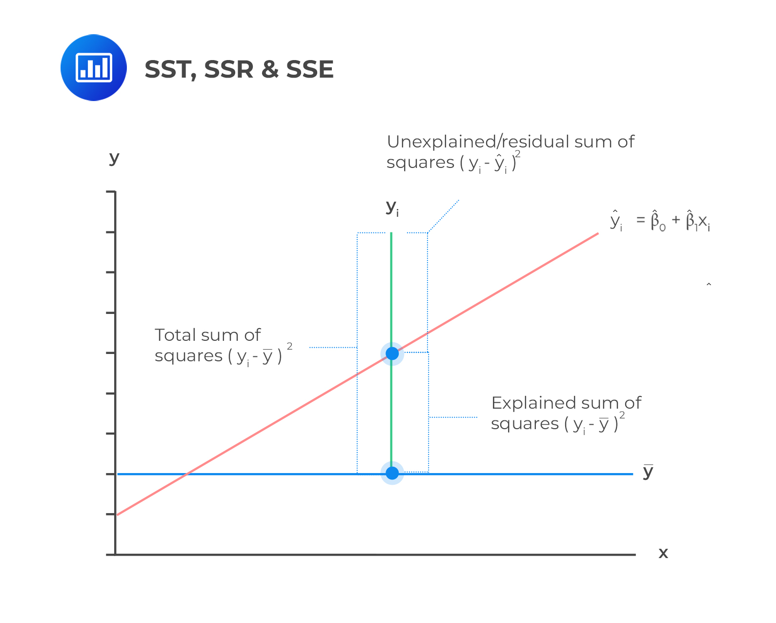
Sum of Squares Total (total variation) is a measure of the total variation of the dependent variable. It is the sum of the squared differences of the actual y-value and mean of y-observations.

$$\text{SST} = \sum_{i=1}^{n}{(Y_i-\bar{Y})^2}$$

The Sum of Squares Total contains two parts:

1. Sum of Square Regression (SSR).
2. Sum of Squares Error (SSE).

Sum of Squares Regression (SSR)

The sum of squares regression is the measure of the explained variation in the dependent variable. It is given by the sum of the squared differences of the predicted y-value (\(\widehat{Y}\)), and mean of y-observations, (\(\bar{Y}\)):

$$\text{SSR} = \sum_{i=1}^{n}{(\widehat{Y}_i-\bar{Y})^2}$$

Sum of Squared Errors (SSE)

The sum of squared errors is also called the residual sum of squares. It is defined as the variation of the dependent variable unexplained by the independent variable. SSE is given by the sum of the squared differences of the actual y-value (\(Y_i\)), and the predicted y-values, (\(\widehat{Y}_i\)).

$$\text{SSE} = \sum_{i=1}^{n}{(Y_i-\widehat{Y}_i)^2}$$

Therefore, the sum of squares total is given by:

$$\begin{align}\text{Sum of Squares Total} &= \text{Explained Variation + Unexplained Variation}\\&= \text{SSR+ SSE}\end{align}$$

The components of the total variation are shown in the following figure.

Coefficient of Determination

The coefficient of determination (\(R^2\)) measures the proportion of the total variability of the dependent variable explained by the independent variable. It is calculated using the formula below:

$$R^2 = \frac{\text{Explained Variation}}{\text{Total Variation}}=\frac{\text{Sum of Squares Regression (SSR)}}{\text{Sum of Squares Total (SST)}}$$

Intuitively we can think of the above formula as:

$$\begin{align}R^2&=\frac{\text{Total Variation-Unexplained Variation}}{\text{Total Variation}}\\ &=\frac{\text{Sum of Squares Total (SST)-Sum of Squared Errors (SSE)}}{\text{Sum of Squares Total}}\end{align}$$

Simplifying the above formula gives:

$$R^2 =1-\frac{\text{Sum of Squared Errors (SSE)}}{\text{Sum of Squares Total (SST)}}$$

Features of Coefficient of Determination (\(R^2\))

\(R^2\) lies between 0 and 1. A high \(R^2\) explains variability better than a low \(R^2\). If \(R^2= 0.01\), only 1% of the total variability can be explained. On the other hand, if \(R^2= 0.90\), over 90% of the total variability can be explained. In a nutshell, the higher the \(R^2\), the higher the explanatory power of the model.

For models with one independent variable, \(R^2\) is calculated by squaring the correlation coefficient between the dependent and the independent variables:

$$R^2=\left(\frac{Cov\left(X,Y\right)}{\sigma_X\sigma_Y}\right)^2$$

Where:

\(Cov\ (X,Y)\) = covariance between two variables, X and Y.

\(\sigma_X\) = standard deviation of X.

\(\sigma_{Y}\) = standard deviation of Y.

Example: Calculating Coefficient of Determination (\(R^2\))

An analyst determines that \(\sum_{i\ =\ 1}^{6}{\left(Y_i-\bar{Y}\right)^2=\ }0.0013844\) and \( \sum_{i\ =\ 1}^{6}\left(Y_i-\widehat{Y}\right)^2= 0.0003206\) from the regression analysis of inflation on unemployment. The coefficient of determination (\(R^2\)) is closest to:

Solution

$$\begin{align}R^2&=\frac{\text{Sum of Squares Total (SST)-Sum of Squarred Errors (SSE) }}{\text{Sum of Squares Total (SST)}}\\ &=\frac{\left(\sum_{i=1}^{n}\left(Y_{i}-\bar{Y}\right)^{2}-\sum_{i=1}^{n}\left(Y_{i}-\widehat{Y}\right)^{2}\right)}{\sum_{i=1}^{n}\left(Y_{i}-\bar{Y}\right)^{2}}\\ &=\frac{0.0013844-0.0003206}{0.0013844}=0.7684=76.84\%\end{align}$$

F-statistic in Simple Regression Model

Note that the coefficient of variation discussed above is just a descriptive value. To check the statistical significance of a regression model, we use the F-test. The F-test requires us to calculate the F-statistic.

The F-test confirms whether the slope (denoted by \(b_i\)) in a regression model is equal to zero. In a typical simple linear regression hypothesis, the null hypothesis is formulated as: \(H_0:b_1=0\) against the alternative hypothesis, \(H_1:b_1\neq 0\). The null hypothesis is rejected if the confidence interval at the desired significance level excludes zero.

The Sum of Squares Regression (SSR) and Sum of Squares Error (SSE) are employed to calculate the F-statistic. In the calculation, both the Sum of Squares Regression (SSR) and Sum of Squares Error (SSE) are adjusted for the degrees of freedom.

The Sum of Squares Regression is divided by the number of independent variables, \(k\), to get the Mean Square Regression (MSR). That is:

$$MSR=\frac{SSR}{k}\ =\ \frac{\sum_{i\ =\ 1}^{n}\left(\widehat{Y}_i-\bar{Y}\right)^2}{k}$$

Since we only have \(k =1\), in a simple linear regression model, the above formula changes to:

$$MSR=\frac{SSR}{1}=\frac{\sum_{i\ =\ 1}^{n}\left(\widehat{Y}_i-\bar{Y}\right)^2}{1}=\sum_{i\ =\ 1}^{n}\left(\widehat{Y}_i-\bar{Y}\right)^2$$

Therefore, in Simple Linear Regression Model, MSR = SSR.

Also, the Sum of Squares Error (SSE) is divided by degrees of freedom given by \(n-k-1\) (this translates to \(n-2\) for simple linear regression) to arrive at Mean Square Error (MSE). That is,

$$MSE=\frac{\text{Sum of Squares Error (SSE)}}{n-k-1}=\frac{\sum_{i=1}^{n}\left(Y_i-\widehat{Y}\right)^2}{n-k-1}$$

For a simple linear regression model,

$$MSE\ =\frac{\text{Sum of Squares Error(SSE)}}{n-2}\ \ =\ \ \frac{\sum_{i\ \ =\ \ 1\ }^{n}\left(Y_i-\widehat{Y}\right)^2}{n-2}$$

Finally, to calculate the F-statistic for the linear regression, we find the ratio of MSR to MSE. That is,

$$ F-statistic\ =\ \frac{MSR}{MSE}\ =\ \frac{\frac{SSR}{k}}{\frac{SSE}{n-k-1}}\ =\ \frac{\frac{\sum_{i=1}^{n}\left(\widehat{Y}_i-\bar{Y}\right)^2}{k}}{\frac{\sum_{i\ =\ 1\ }^{n}\left(Y_i-\widehat{Y}\right)^2}{n-k-1}} $$

For simple linear regression, this translates to:

$$F-statistic=\frac{MSR}{MSE}=\frac{\frac{SSR}{k}}{\frac{SSE}{n-k-1}}\ =\ \frac{\frac{\sum_{i=1}^{n}\left(\widehat{Y}_i-\bar{Y}\right)^2}{1}}{\frac{\sum_{i\ =\ 1\ }^{n}\left(Y_i-\widehat{Y}\right)^2}{n-2}}\ =\ \frac{\sum_{i\ =\ 1}^{n}\left(\widehat{Y}_i-\bar{Y}\right)^2}{\frac{\sum_{i\ =\ 1}^{n}\left(Y_i-\widehat{Y}\right)^2}{n-2}}$$

The F-statistic in simple linear regression is F-distributed with \(1\) and \(n-2\) degrees of freedom. That is,

$$\frac{MSR}{MSE}\sim F_{1,n-2}$$

Interpretation of F-test Statistic

A large F-statistic value proves that the regression model is effective in its explanation of the variation in the dependent variable and vice versa. On the contrary, an F-statistic of 0 indicates that the independent variable does not explain the variation in the dependent variable.

We reject the null hypothesis if the calculated value of the F-statistic is greater than the critical F-value.

It is worth mentioning that F-statistics are not commonly used in regressions with one independent variable. This is because F-statistic is equal to the square of the t-statistic for the slope coefficient, which implies the same thing as the t-test.