Cash Flow Additivity

A timeline is a physical illustration of the amounts and timing of cashflows associated with an investment project. For cashflows that are regular and of equal amounts, the standard annuity formula or the financial calculator can be used. However, a timeline is preferred for irregular, unequal, or both cashflows.

Remember that the general formula that relates the present value and the future value of an investment is given by:

$$ FV_N=PV(1+r)^N $$

Where:

\(PV\) = Present value of the investment.

\(FV_N\)= Future value of the investment N periods from today.

\(r\) = Rate of interest per period.

We can represent this in a timeline:

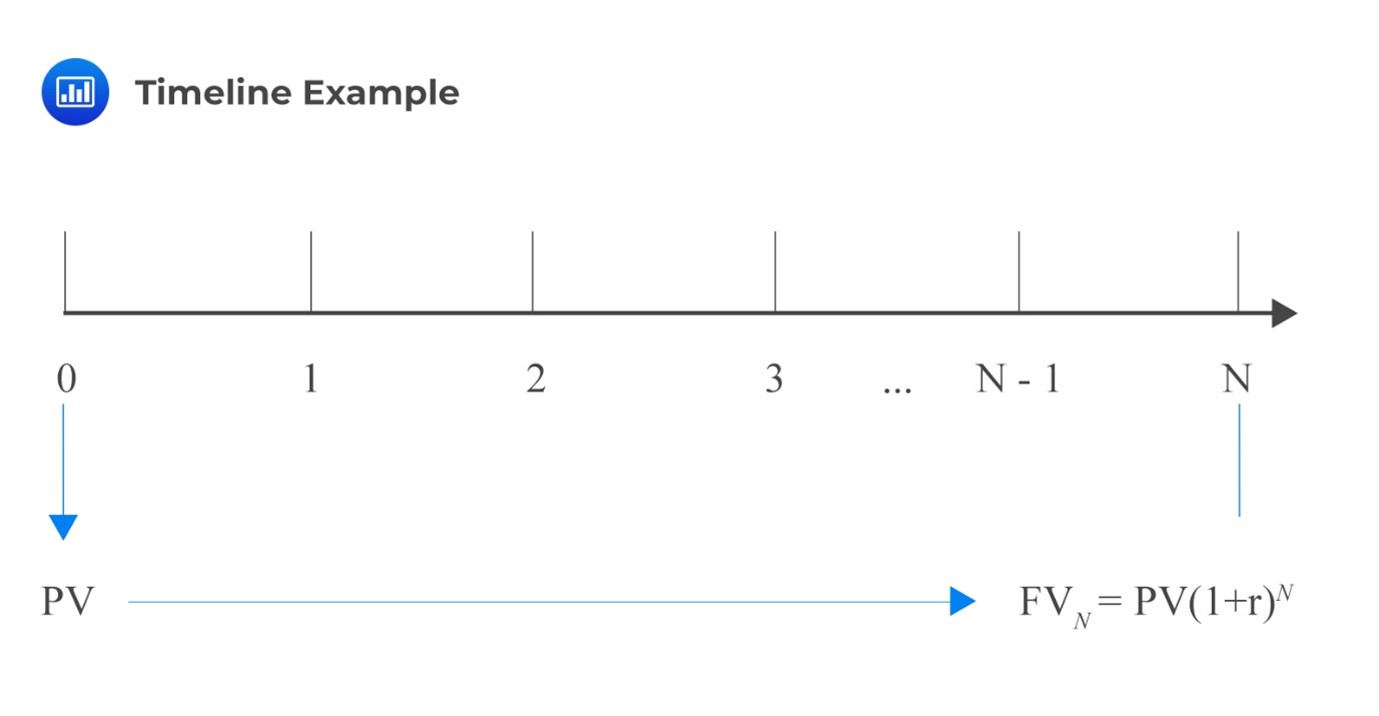
In a particular timeline, a time index, \(t\), represents a particular point in time, a specified number of periods from today. Therefore, the present value is the investment amount today (t = 0), and by using this amount, we can calculate the future value (t = N). Alternatively, we can use the future value to calculate the present value.

The above argument can be written in terms of the present value. That is:

$$ PV=FV_N (1+r)^{-N} $$

Example: Applying a Timeline to Model Cashflows

A fixed-income investor receives a series of payments, each amounting to $6,500, set to be received in perpetuity. Payments are to be made at the end of each year, starting at the end of year 4. If the discount rate is 9%, then what is the present value of the perpetuity at \(t\) = 0?

Solution

We would then draw a timeline to understand the problem better:

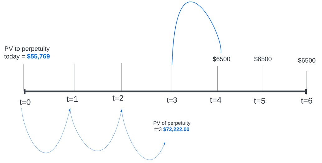
Here, we can see that the investor is receiving $6,500 in perpetuity. Recall that the PV of aperpetuity is given by:

$$ \text{PV of a perpetuity}=\frac {C}{r} $$

So, in this case:

$$ PV_3=\frac {\$6,500}{9\%}=\$72,222 $$

This is the value of the perpetuity at \(t\) = 3, so we need to discount it for three more periods to get the value at \(t\) = 0. Using the formula:

$$ PV_0=FV_N (1+r)^{-N} $$

The PV at time zero is \(\frac {\$72,222}{(1+0.09)^3} =\$55,769 \)

Why is the Use of a Timeline Recommended?

There are many instances in real life when cashflows are uneven. A good example is a pension contribution that varies with age. Applying one of the basic time value formulae is impossible in such cases. You are advised to draw a timeline even if the question appears relatively straightforward. It will help you understand the question structure better. A timeline also helps candidates add cashflows indexed to the same period and apply the value additivity principle.

Cashflow Additivity Principle

According to the cashflow additivity principle, the present value of any stream of cashflows indexed at the same point equals the sum of the present values of the cashflows. This principle has different applications in time value of money problems. Besides, this principle can be applied to in different economic scenarios.

Application of Cashflow Additivity

Investing in Different Currencies

The principle of cash flow additivity can be applied to scenarios involving different currencies by converting all cash flows to a common currency using the appropriate exchange rates. Doing so allows us to compare and combine cash flows from different currencies and make investment decisions based on their combined value.

For example, suppose we have two investment opportunities, one in US dollars and one in Japanese yen. In that case, we can convert the expected cash flows from the Japanese yen investment into US dollars using the appropriate exchange rates. Then, we can compare the combined value of the two investments and decide based on their relative values.

Dealing with different currencies assumes continuous compounding. Recall that the present value of a continuous compounding is given by:

$$ PV=FV_N e^{-Nr_s} $$

Example: Applying the Cash Flow Additivity Principle

Consider an investor with USD 2,000 who wants to invest it for three months. The investor can choose between two options: investing in the US government debt or German government debt.

Option 1: Investing in US Government Debt

The investor can invest his USD 2,000 in a three-month US Treasury bill. This means that he lends the government USD 2,000, and it promises to pay him back with interest in three months. The interest is 3%, so after three months, he will receive:

Recall that,

$$ FV=2,000 \times e^{0.03 \times \frac {3}{12}}=\text{USD } 2,015 $$

Option 2: Investing in German Government Debt

The investor chooses to invest in German government debt. To do this, the investor must convert his USD 2,000 into Euros at the current exchange of EUR/USD = 0.92 (1 USD =0.92EUR). This means that the investor will receive \((2,000 \times 0.92)=\text{EUR } 1840\). He can then lend this money to the German government by investing in a three-month German Treasury bill. Assuming the interest rate is 0.06 percent, after three months, the investor will receive:

$$ \begin{align*}
FV & =\text{EUR } 1840 \times e^{0.06 \times \frac {3}{12}} \\
& =\text{EUR } 1,867.81 \end{align*} $$

Assuming the investor wants his money in US dollars, we need to convert the EUR1867.81 back into USD at the forward exchange rate of USD/EUR = 1.0788. This means that the investor will receive:

\(\frac {\text{EUR }1,867.81 \times \text{USD }1.0788}{1 \text{ EUR}}=\$2,014.99 \approx 2,015\)

Both options give you the same amount of money after three months: USD 2,015. The difference is that one option involves investing in US dollars, and the other involves converting your money into Euros and back into US dollars.

The forward exchange rate of 1.0788 USD/EUR is important because it determines how much money you, the investor, will receive when converting your Euros back into US dollars. If this rate differs from 1.0788, there would be an arbitrage opportunity in converting Euros to dollars.

More on foreign exchange rates will be discussed later in the curriculum.

Implied Forward Rates

Consider two zero-coupon bonds. Bond A has a maturity of two years and a yield of 2% per annum, while bond B has a maturity of four years and a yield of 3%. An investor, who doesn’t seek to take advantage of price differences and is risk-neutral, has $1,000 to invest. The investor has two investment options that earn the same return.

Option 1: The investor can put their money into bond B now, which has an annual yield of 3%, and will pay out at the end of the four years. The Future Value (FV) of this investment in four years, using the formula for compound interest, is:

$$ FV_4=PV_0 (1+r_4)^4=1000(1.03)^4=1,125.51 $$

Option 2: Alternatively, the investor can initially invest in bond A and, after two years, reinvest the proceeds at a forward rate \(F_{2,2}\) which represents a two-year forward rate starting in year two.

By the principle of cash flow additivity, a risk-neutral investor will not prefer one option over the other – they are indifferent between Options 1 and 2. This is because the Future Values of both investments at the end of four years should be the same:

$$ FV_4=PV_0 (1+r_4)^4=PV_0 (1+r_2)(1+F_{2,2}) $$

In this scenario, this simplifies to:

$$ 1,125.51=1,000(1.02)^2 (1+F_{2,2}) $$

Solving this equation for the forward rate gives:

$$ \Rightarrow F_{2,2}=\frac {1,125.51}{1,000(1.02)^2}-1=8.18\% $$

Therefore, to prevent arbitrage opportunities, the forward rate \(F_{2,2}\) should be set to 8.18%. This ensures that there is no potential for risk-free profits, maintaining market efficiency.

Cashflow Additivity and Option Pricing

Cash flow additivity can be used to determine the fair price of an option contract. An option contract gives the buyer the right, but not the obligation, to buy (call) or sell (put) an underlying asset at a specified price within a certain period.
Cash flow additivity allows investors to compare different strategies and determine a no-arbitrage price for a financial instrument.

Example: Illustrating Cashflow Additivity in Call Option

Consider a stock that costs $100 now. Its price might increase by 30% to $130 or decrease by 15% to $85 in one year.

Let’s say an investor wants to sell a call on the stock that gives the buyer the right, but not the obligation, to purchase the asset for $120. The principle of cash flow additivity can be used to determine the contract’s no-arbitrage price.

If the stock price goes up, the contract is worth \(c_1^u=10\). That’s because the buyer can use the contract to buy the asset for $120 and then sell it for $130, making a profit of $10. But if the price goes down, the contract is worth nothing. The buyer wouldn’t want to use the contract to buy the asset for $120 when they could just buy it for $85 without the contract.

The underlying argument here is that the value of the option is each movement of the stock option may be used to construct a risk-free portfolio (the value of the portfolio is the same in both scenarios).

Denote the initial value of the call option by \(c_0\), which we wish to determine using cash flow additivity and no-arbitrage pricing. Also, denote the value of the portfolio at \(t=0\) by \(V_0\), when the stock price increases by \(V_1^u\) and when the stock price decreases by \(V_1^d\)

Assume that at \(t=0\) creates a risk-free portfolio by selling a call option at \(c_0\) and buying 0.22 units of underlying assets. Then, the value of the portfolio at inception is:

$$ V_0=0.22 \times 100-c_0 $$

This portfolio is called a replicating portfolio because it is designed to create a matching future cash flow stream to that of a risk-free asset.

Similarly, in each scenario of stock price decrease and increase:

$$ \begin{align*} V_1^u & =0.22 \times 130-10=18.89 \\
V_1^d & =0.22 \times 85-0=18.89 \end{align*} $$

Intuitively, the value replicating portfolio equals 18.89, whether the stock prices rise or decline. As such, the replicating portfolio is risk-free and can be discounted as a risk-free asset. Assuming that risk-free rate is r = 2.5%, then:

$$ \begin{align*}
V_0 & =V_1^u (1+r)^{-1}=V_1^d (1+r)^{-1} \\
& =18.89(1.025)^{-1}=18.43 \end{align*} $$

At this point, we can calculate the value of \(c_0\) rearranging the initial portfolio value equation:

$$ \begin{align*} V_0 & =0.22 \times 100-c_0 \\
\Rightarrow 18.43 & =0.22 \times 100-c_0 \\
\therefore c_0 & =3.57 \end{align*} $$

As such, the fair price of the call option is $3.57, which the seller expects to receive from the buyer.

Question

The current USD/CHF exchange rate is 0.9. The risk-free interest rates for one year are 2% for the US dollar and 1% for the Swiss franc. Which of the following one-year USD/CHF forward rates would best prevent arbitrage opportunities?

1. USD/CHF 0.909.
2. USD/CHF 0.099.
3. USD/CHF 0.891.

Solution

The correct Answer is A.

Dealing with different currencies assumes continuous compounding. Recall that the future value of a continuous compounding is given by:

$$ FV=PV_N e^{-Nr_s} $$

So,

In one year, a single unit of Swiss franc invested is:

$$ e^{0.01}=\text{CHF } 1.0101 $$

In one year, a single unit of Swiss Franc converted to US dollars and then invested risk-free is worth;

$$ 0.9e^{0.02}=\text{USD } 0.9182 $$

Therefore, to convert USD 0.9182 into CHF 1.0101 requires a forward exchange rate of:

$$ \frac {0.9182}{1.0101}=\text {USD/CHF } 0.909 $$