Analysis of Variance (ANOVA)

The sum of squares of a regression model is usually represented in the Analysis of Variance (ANOVA) table. The ANOVA table contains the sum of squares (SST, SSE, and SSR), the degrees of freedom, the mean squares (MSR and MSE), and F-statistics.

The typical format of ANOVA is as shown below:

$$
\begin{array}{l|c|c|c|c}
\begin{array}{l}
\textbf { Source of } \\
\textbf { Variation }
\end{array} & \begin{array}{l}
\textbf { Sum of } \\
\textbf { Squares }
\end{array} & \begin{array}{l}
\textbf { Degrees of } \\
\textbf { Freedom }
\end{array} & \textbf { Mean Squares } & \textbf { F-statistic } \\
\hline \begin{array}{l}
\text { Regression } \\
\text { (Explained) }
\end{array} & \text { SSR } & 1 & \text { MSR }=\frac{S S R}{1} & F=\frac{M S R}{M S E} \\
\hline \begin{array}{l}
\text { Residual } \\
\text { Eror } \\
\text { (Unexplained) }
\end{array} & \text { SSE } & \text { N_-2 } & \text { MSE }=\frac{S S E}{n-2} & \\
\hline \text { Total } & \text { SST } & \mathrm{N}-1 & & \\
\end{array}
$$

Standard Error of Estimate

Standard Error of Estimate, \(S_e\) or \(SEE\), is alternatively referred to as the root mean square error or standard error of regression.  It measures the distance between the observed dependent variables and the dependent variables predicted by the regression model. The Standard Error of Estimate is easily calculated from the ANOVA table using the following formula:

$$\text{Standard Error of Estimate}(S_e)=\sqrt{MSE}=\sqrt{\frac{\sum_{i\ =\ 1}^{n}\left(Y_i-\hat{Y}\right)^2}{n-2}}$$

The standard error of estimate, coefficient of determination, and F-statistic are the measures that can be used to gauge the goodness of fit of a regression model. In other words, these measures are used to tell the extent to which a regression model syncs with data.

The smaller the Standard Error of Estimate is, the better the fit of the regression line. However, the Standard Error of Estimate does not tell us how well the independent variable explains the variation in the dependent variable.

Example: Calculating the Standard Error of Estimate (\(S_e\))

An analyst is using regression analysis to forecast inflation given unemployment data from 2011 to 2020. The following table shows the relevant data from 2011 to 2020:

$$\small{\begin{array}{c|c|c}\textbf{Year} & \textbf{Unemployment Rate} & \textbf{Inflation rate}\\ \hline 2011 & 6.1\% & 1.7\%\\ \hline 2012 & 7.4\% & 1.2\%\\ \hline 2013 & 6.2\% & 1.3\%\\ \hline 2014 & 6.2\% & 1.3\%\\ \hline 2015 & 5.7\% & 1.4\%\\ \hline 2016 & 5.0\% & 1.8\%\\ \hline 2017 & 4.2\% & 3.3\%\\ \hline 2018 & 4.2\% & 3.1\%\\ \hline 2019 & 4.0\% & 4.7\%\\ \hline 2020 & 3.9\% & 3.6\%\\ \end{array}}$$

The analyst has estimated the linear regression equation for inflation and unemployment as:

$$\hat{Y} = 0.070953-0.90405X_i$$

Calculate the standard error of estimate (SEE).

Solution

Consider the following table:

$$\small{\begin{array}{c|c|c|c|c|c}\textbf{Year} & {\textbf{Unemployment}\\ \bf{X_i}} & {\textbf{Inflation}\\{Y_i}} & {\textbf{Predicted}\\ \textbf{Inflation value}\\ \widehat{Y_i}} & {\textbf{Regression}\\ \textbf{ residual}\\{Y_i}-\widehat{Y_i}} & {\textbf{Squared}\\ \textbf{residual} \\Y_i-\widehat{Y_i}^{2}}\\ \hline 2011 & 6.1\% & 1.7\% & 0.0162699 & 0.0002301 & 0.0000001\\ \hline 2012 & 7.4\% & 1.2\% & 0.0043364 & 0.0077636 & 0.0000603\\ \hline 2013 & 6.2\% & 1.3\% & 0.0152754 & -0.0020754 & 0.0000043\\ \hline2014 & 6.2\% & 1.3\% & 0.0152754 & -0.0020754 & 0.0000043\\ \hline 2015 & 5.7\% & 1.4\% & 0.0192533 & -0.0049533 & 0.0000245\\ \hline 2016 & 5.0\% & 1.8\% & 0.0262145 & -0.0086145 & 0.0000742\\ \hline 2017 & 4.2\% & 3.3\% & 0.0331757 & -0.0001757 & 0.0000000\\ \hline 2018 & 4.2\% & 3.1\% & 0.0331757 & -0.0023757 & 0.0000056\\ \hline 2019 & 4.0\% & 4.7\% & 0.0351646 & 0.0121354 & 0.0001473\\ \hline 2020 & 3.9\% & 3.6\% & 0.0361591 & 0.0001409 & 0.0000000\\ \hline\textbf{Sum}& & & & & \textbf{0.0003206}\\ \end{array}}$$

$$\text{SEE}=\bigg[\frac{\sum_{i=1}^n(Y_i-\widehat{Y_i})^2}{n-2}\bigg]^{\frac{1}{2}}$$

Where:

• \(\widehat{Y_1}=\widehat{b_0}+\widehat{b_1}X_i\)
• \(\widehat{b_0}=0.070953\)
• \(\widehat{b_1}=-0.90405\)

$$\sum_{i=1}^n(Y_i-\widehat{Y}_1)^2=0.0003206$$

$$\text{SEE}=\bigg[\frac{0.0003206}{10-2}\bigg]^{\frac{1}{2}}=0.00633$$

Note: CFA Insititute will most likely not require you to do such a long calculation. However, it is important to understand the steps you need to take to go from raw data to the SEE.

Example: Calculating and Interpreting F-Statistic

The completed ANOVA table for the regression model of inflation rate against unemployment rate over 10 years is given below:

$$
\begin{array}{c|c|c|c}
 \textbf { Source of variation } & \textbf { Sum of squares } & \textbf { Degrees of freedom } & \begin{array}{l}
\textbf { Mean sum of } \\
\textbf { squares }
\end{array} \\
\hline \begin{array}{c}
\text { Regression } \\
\text { (Explained) }
\end{array} & 0.004249 & 1 & 0.004249 \\
\hline \begin{array}{c}
\text { Residual Error } \\
\text { (Unexplained) }
\end{array} & 0.002686 & 8 & 0.0001492 \\
\hline \text { Total } & 0.006935 & 9 & \\
\end{array}
$$

a) Use the above ANOVA table to calculate the F-statistic.

b) Test the hypothesis that the slope coefficient is equal to at a 5% significance level.

Solution

a)

$$\begin{align} F &=\frac{\text{Mean Regression Sum of Squares (MSR)}}{\text{Mean Squared Error(MSE)}}\\ &=\frac{0.004249}{0.0001492}=28.48\end{align}$$

b)

We are testing the null hypothesis \(H_0:b_1=0\) against the alternative hypothesis \(H_1:\ b_1\ \neq 0\). The critical F-value for \(k = 1\) and \(n-2 = 8\) degrees of freedom at a 5% significance level is roughly 5.32. Note that this is a one-tail test and therefore, we use the 5% F-table.

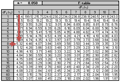
Remember that the null hypothesis is rejected if the calculated value of the F-statistic is greater than the critical value of F. Since \(28.48 > 5.32\), we reject the null hypothesis and arrive at the conclusion that the slope coefficient is significantly different from zero.

Notice that we also rejected the null hypothesis in the previous examples. We did so because the 95% confidence interval did not include zero.

An F-test duplicates the t-test in regard to the slope coefficient significance for a linear regression model with one independent variable. In this case, \(t^2={2.306}^2\approx 5.32\). Since F-statistic is the square of the t-statistic for the slope coefficient, its inferences are the same as the t-test. However, this is not the case for multiple regressions.

Question

Consider the following analysis of variance (ANOVA) table:

$$
\begin{array}{l|c|c|c}
 \textbf { Source of Variation } & \textbf { Degrees of Freedom } & \begin{array}{c}
\textbf { Sum of } \\
\textbf { Squares }
\end{array} & \textbf { Mean Sum of Squares } \\
\hline \text { Regression (Explained) } & 1 & 1,701,563 & 1,701,563 \\
\hline \begin{array}{l}
\text { Residual Error } \\
\text { (Unexplained) }
\end{array} & 3 & 106,800 & 13,350 \\
\hline \text { Total } & 4 & 1,808,363 & \\
\end{array}
$$

The value of \(R^2\) and the F-statistic for the test of fit of the regression model are closest to:

1. 6% and 16.
2. 94% and 127.
3. 99% and 127.

Solution

The correct answer is B.

$$R^2=\frac{\text{Sum of Squares Regression (SSR)}}{\text{Sum of Squares Total (SST)}}=\frac{1,701,563}{1,808,363}=0.94=94\%$$

$$F=\frac{\text{Mean Regression Sum of Squares (MSR)}}{\text{Mean Squared Error (MSE)}}=\frac{1,701,563}{13,350}=127.46\approx 127$$