Introduction to Credit Risk Modeling and Assessment

After completing this reading, you should be able to:

• Explain the capital adequacy, asset quality, management, earnings, and liquidity (CAMEL) system used for evaluating the financial condition of a bank.
• Describe quantitative measurements and factors of credit risk, including probability of default, loss given default, exposure at default, expected loss, and time horizon.
• Estimate capital adequacy ratio of a financial institution.
• Describe the judgmental approaches, empirical models, and financial models to predict default.55
• Apply the Merton model to calculate default probability and the distance to default and describe the limitations of using the Merton model.
• Compare and contrast different approaches to credit risk modeling, such as those related to the Merton model, Credit Risk Plus (CreditRisk+), CreditMetrics, and the Moody’s-KMV model.
• Apply risk-adjusted return on capital (RAROC) to measure the performance.

The Evolution of Risk Management

Credit is an essential tool in both the private and public sectors, crucial for liquidity and funding in economic activities, daily operations, and long-term investments. Its use dates back to early civilization, but recent decades have seen significant changes in the volume of credit, the channels through which it’s provided, the types of available credit, and the regulatory framework governing its provision.

Credit risk, the likelihood that a borrower will not meet their debt obligations, has become a major concern for organizations involved in credit transactions and their supervision. This risk is traditionally associated with financial institutions like banks, but it’s also relevant in the non-financial sector, where firms often extend credit to customers and receive it from suppliers. The financial stability of these partners is crucial to avoid severe financial and operational difficulties.

Data from the Bank of International Settlements shows a substantial expansion of credit in the Eurozone and the USA from 2000 to 2016. In the Eurozone, total credit increased by 105.5% to 17,481 billion euros, while in the USA, it grew by 123.5% to over $28,200 billion. When compared to GDP, the growth seems more moderate, but private debt to the non-financial sector exceeds 150% of GDP in both regions. The composition of this debt varies: in the Eurozone, credit to non-financial corporations predominates, while in the USA, household credit is higher.

The banking sector’s contribution to providing private credit has evolved differently in these regions. In the Eurozone, banks’ share in total credit reduced from 63% in 2000 to 56.4% in 2016, while in the USA, banks contribute around 35% of total credit. The use of new financial instruments like credit derivatives (e.g., credit default swaps, collateralized debt obligations) and emerging financing systems (social lending, peer-to-peer lending, crowdfunding) has introduced new challenges in monitoring credit expansion and assessing risks.

Credit risk management, a complex process involving analysis, assessment, and monitoring of credit risk in financial transactions, has undergone dramatic changes over the past decades. These changes are most evident in financial institutions and credit risk management solution providers, but they indirectly affect all organizations exposed to credit risk. The multifaceted nature of managing credit risk presents various regulatory, methodological, and technical challenges, continually evolving in response to the financial landscape.

The evolution of credit risk management, from empirical models like the Basel Accord to modern analytical tools such as the FICO score, underscores the complexity of assessing creditworthiness. These advancements play a critical role in informing the Management aspect of the CAMEL system—a framework used to evaluate a bank’s health across five domains: Capital Adequacy, Asset Quality, Management, Earnings, and Liquidity. Effective management of credit risk is vital, as it affects a bank’s capital structure, asset integrity, profitability, and ability to meet its cash flow needs, which are all assessed under the CAMEL rating system.

The CAMEL Rating System

The CAMEL rating system stands as a testament to the evolution of financial oversight and prudent banking regulation. Developed in the U.S. in the early 1970s, the system was initially a supervisory tool used by the Federal Reserve and later adopted by other regulatory bodies, including the Federal Deposit Insurance Corporation (FDIC). It was designed to provide a systematic method for evaluating the strength and stability of banks and to ensure that they could withstand economic stress. This model has since been embraced internationally, with variations, as a standard for assessing the health of banking institutions.

The acronym CAMEL represents the five critical dimensions of a bank’s financial health: Capital Adequacy, Asset Quality, Management, Earnings, and Liquidity. Each element is scored on a scale, typically from one to five, with one indicating the strongest performance and five indicating the weakest. The composite score is used to make informed decisions about a bank’s regulatory oversight level, including the frequency of inspections and the need for corrective measures.

The significance of the CAMEL system is rooted in its comprehensive approach to risk assessment. It provides a snapshot of a bank’s operational health and its resilience to financial fluctuations. By evaluating these five components, regulators can identify potential problems before they become systemic issues. For example, the 1980s savings and loan crisis highlighted the need for robust risk management practices, where a more proactive application of the CAMEL system could have mitigated the impact.

In the modern financial landscape, the CAMEL system remains an indispensable tool. It aids in safeguarding the stability of the banking sector by ensuring that institutions have sufficient capital buffers, maintain high-quality assets, are managed effectively, generate sustainable earnings, and have adequate liquidity to handle unexpected shocks. As such, the CAMEL rating system not only serves as a barometer of individual bank health but also as a gauge for the broader financial ecosystem’s stability.

Capital Adequacy Ratio

Capital Adequacy Ratio (CAR) is a measure used to assess a financial institution’s strength and stability, representing the ratio of its capital to its risk-weighted assets. 

CAR assesses a bank’s capital relative to its risk exposure. Capital acts as a cushion against losses, so a bank with higher capital adequacy is better positioned to withstand financial distress. For example, if Bank A has a capital adequacy ratio of 10% and Bank B only 5%, Bank A is considered more robust against potential losses. In the 2008 financial crisis, banks with higher capital adequacy were more resilient. 

The concept of CAR emerged from international efforts to establish standardized guidelines for financial institutions, beginning with the Basel I Accord in 1988 and evolving through Basel II, which is currently active. These accords aim to formalize the processes for measuring, managing, and reporting credit risk exposures.

CAR is calculated as:

$$\text{CAR} = \frac{\text{Tier 1 Capital}+\text{Tier 2 Capital}}{\text{Risk-weighted assets}}$$

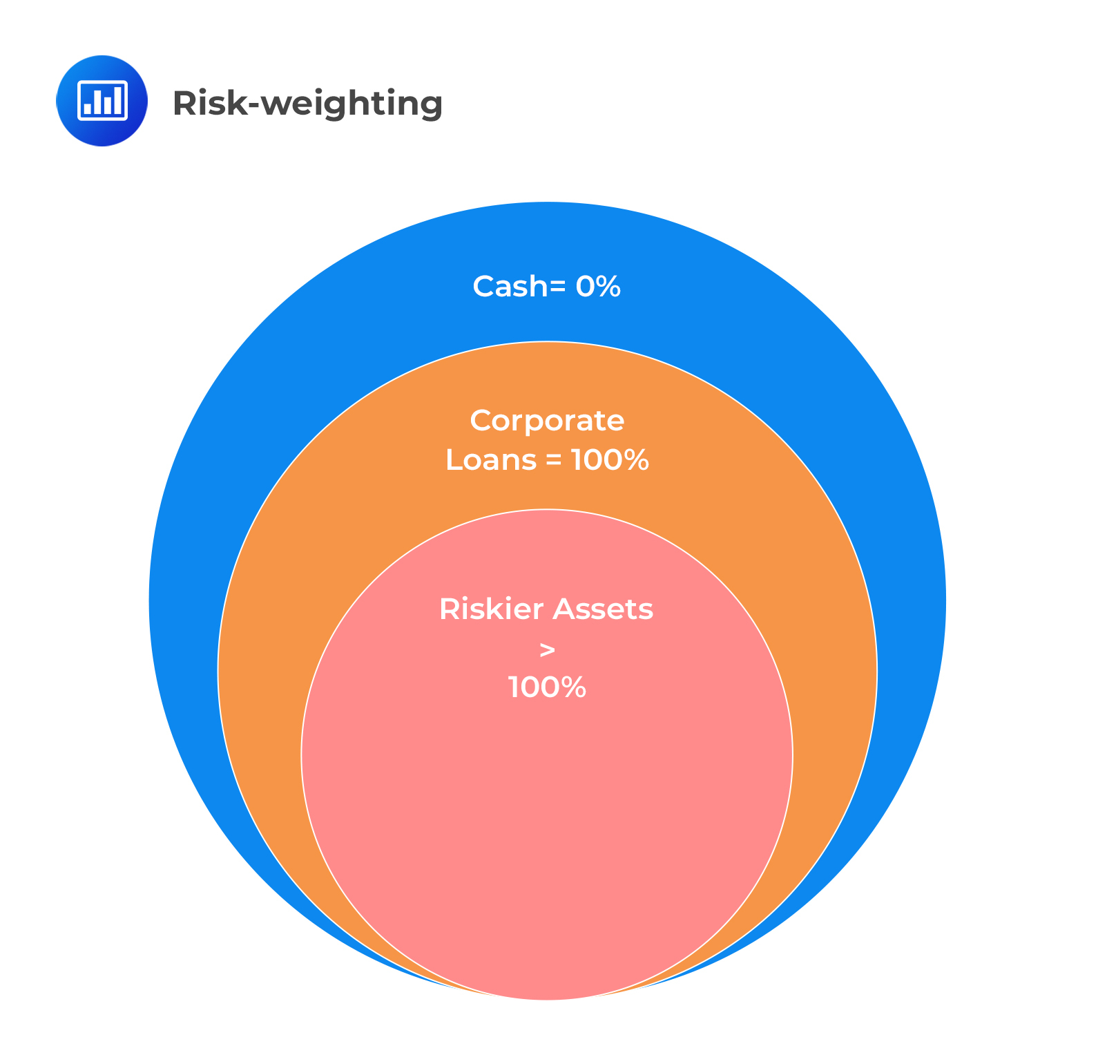
where \(\alpha\) is the minimum requirement set by the regulatory authority (e.g., 8% under Basel II). Risk-weighted assets (RWA) are calculated by assigning different risk weights to the assets based on their risk profile, with higher-risk assets requiring more capital.

The requirement to maintain a certain CAR ensures that financial institutions have enough capital to absorb potential losses, promoting the overall stability and reliability of the financial system. Capital adequacy is not just about the quantity but the quality of capital; tier 1 capital, such as common equity, is more valued than tier 2 capital, like subordinated debt.

Asset Quality
This aspect examines the quality of the bank’s assets, especially its loan portfolio. It focuses on the proportion of non-performing loans to total loans. A higher ratio suggests poorer asset quality, which can erode earnings and capital. For instance, if a significant portion of a bank’s loan portfolio is in default and not accruing interest, the bank’s asset quality would be considered low. Hypothetically, if a bank’s loans are predominantly in a sector experiencing an economic downturn, such as the real estate market post-2007, this would negatively impact its asset quality.

Management
Effective management is key to a bank’s success and is judged on the bank’s ability to identify, measure, monitor, and control risks, and to ensure the bank operates safely. For example, if a bank’s management team successfully navigates through a financial downturn by adjusting credit policies and managing costs, it demonstrates strong management. Conversely, if a new management team fails to comply with regulatory requirements, it indicates weak management.

Earnings
A bank’s earnings, derived from net interest margins, fees, and investments, reflect its ability to generate profit. Consistently strong earnings contribute to capital growth and buffer against losses. Consider JPMorgan Chase’s reported net income in 2019, which showed robust earnings and, hence, financial health. Conversely, if a bank reports volatile or declining earnings, it may be at risk. For example, a hypothetical bank that relies heavily on a single type of fee income may be vulnerable if regulations change to limit those fees.

Liquidity
Liquidity measures a bank’s capacity to meet its financial obligations without incurring substantial losses. It involves evaluating liquid assets and the stability of funding sources. For instance, during the 2008 crisis, banks with strong liquidity, like Wells Fargo, were able to function more effectively than those with less liquidity. A bank’s liquidity can also be strained if it has a high ratio of loans to deposits or if it heavily relies on short-term funding, which can disappear quickly in a crisis.

The CAMELS rating system uses a numeric scale to evaluate each of the six components (Capital Adequacy, Asset Quality, Management, Earnings, Liquidity, and Sensitivity to Market Risk). Here’s a bit more detail on the scoring scale:

• Score 1 (Excellent): A bank rated ‘1’ in any component is considered to be in the strongest condition. It demonstrates excellent performance and management in the respective area, showing minimal risk and strong resilience to external shocks.
• Score 2 (Good): A ‘2’ rating indicates a bank is fundamentally sound. While there may be modest weaknesses, they are not significant enough to pose substantial risks, and the bank is generally stable and well-managed.
• Score 3 (Fair): A bank receiving a ‘3’ rating exhibits some operational or financial weaknesses. While these are not immediately threatening, they could lead to some vulnerability if not properly addressed. A score of 3 often triggers more regulatory attention and potential need for improvements.
• Score 4 (Marginal): This rating suggests significant weaknesses and financial or managerial deficiencies. A bank rated ‘4’ is susceptible to failure if these problems are not resolved. Regulatory action and close monitoring are usually required.
• Score 5 (Poor): A ‘5’ indicates a bank in critical condition with a high probability of failure. The institution has serious financial, managerial, or operational issues that require immediate attention and corrective measures.

It’s important to understand that these scores are relative and can be influenced by various factors, including economic conditions, changes in the market, and regulatory changes. The scores are not static and can change over time as a bank’s situation evolves.

Credit and Uncertainty

Credit serves as a fundamental mechanism in economic activities, allowing financial units to utilize future income for current expenditures. This essential function of credit, however, is intertwined with inherent uncertainties. Lending institutions are well aware that a portion of their clients will face challenges or fail to meet their loan obligations. Therefore, it’s crucial for these institutions to effectively navigate this uncertainty, employing predictive tools and techniques to assess the creditworthiness of potential customers accurately.

In the realm of credit, uncertainties manifest in various forms, each with its unique implications:

1. Strategic uncertainty: This type of uncertainty stems from limited knowledge about the borrower’s true intentions and character. Two main issues arise here:
   • Adverse selection: This occurs when the risk of credit is mirrored in the interest rates, leading to higher-risk borrowers being more attracted to credit offers. It creates a cycle where increased risk drives away lower-risk borrowers.
   • Moral hazard: This arises when borrowers, facing unfavorable borrowing terms, are pushed toward higher risk and potential insolvency. For example, the reliance on credit cards as a last-resort lending solution can exacerbate this issue.
2. Occasional uncertainty: This form of uncertainty emerges from unpredictable external factors beyond the borrower’s control. Job losses, economic crises, or even natural disasters can drastically affect a borrower’s repayment ability.

• Cognitive uncertainty: This is related to a borrower’s misperception of their financial status, often leading to irrational financial behaviors. Examples include consumers incurring expenses beyond their means and accumulating debt through high-interest credit cards.

Risk Factors in Credit Decisions

• Credit institutions face numerous risk factors when making lending decisions:
  • Collateral value depreciation: The decrease in the value of assets pledged as security.
  • Over-indebtedness: When a borrower’s debt burden becomes unsustainable.
  • Inadequate assessment: Poor evaluation of a borrower’s solvency, liquidity, and qualitative factors affecting repayment ability.
  • Inconsistent collateral guidelines: Variability in applying collateral and guarantee standards across different loan types.
  • Local discrepancies in loan approval: Differences in loan approval criteria due to local practices or specific authorization techniques.
  • Management and budgeting practices: Weak financial management and lack of effective budgetary control.
  • Misuse of loan funds: Using loans for purposes other than those approved.
  • Loan duration: The risk associated with the term of the loan, with longer durations typically being riskier.
  • Legal and documentation risks: Errors, omissions, or legal misunderstandings in loan agreements.
  • Lack of insurance: Absence of coverage for unforeseen events affecting the borrower’s financial stability.

In conclusion, a comprehensive understanding of the various uncertainties and risk factors is paramount in the field of credit risk management. This involves not only a quantitative analysis of potential risks but also a qualitative assessment of the borrower’s situation and the broader economic environment. Such knowledge is vital for professionals aiming to manage credit risk effectively, particularly those preparing for roles as Financial Risk Managers.

Elements of Credit Risk Modeling

In the realm of financial risk management, credit risk modeling serves a pivotal role. Its primary objective is to estimate the expected loss (EL) for a loan over a designated period, commonly set to one year to align with standard financial reporting intervals. This estimation hinges on three integral components: Probability of Default (PD), Exposure at Default (EAD), and Loss Given Default (LGD).

$$EL = PD\times EAD \times LGD$$

Understanding Probability of Default (PD)

The Probability of Default (PD) is a metric that quantifies the likelihood of a borrower failing to meet loan payments within the specified analysis period. The standard benchmark for defining a default event includes scenarios where payment delays exceed 90 days. However, more nuanced definitions may take into account other elements such as the due amount. PD estimation is typically achieved through credit scoring or rating models that analyze various factors related to the borrower’s status. For example, a borrower’s credit history, current debt levels, and prevailing market conditions are all critical factors that influence PD.

Exposure at Default (EAD)

Exposure at Default (EAD) refers to the total amount due at the time of default. Contrary to PD, EAD is more dependent on the characteristics of the loan rather than the borrower. Fixed-payment loans, such as bonds, offer a straightforward calculation of EAD. In contrast, variable-payment loans, like credit card debts, present a more complex scenario for estimating EAD. For instance, a credit card account with fluctuating balances demands a dynamic approach to ascertain the accurate EAD.

Loss Given Default (LGD)

The Loss Given Default (LGD) represents the proportion of the EAD that is unrecoverable post-default. LGD values typically range from 0 to 100% and are inversely related to the recovery rate (100% minus LGD). LGD is influenced by a mix of factors, including the nature of the borrower, the loan’s specific attributes, and the overarching macroeconomic environment. For corporate loans, variables like the company’s size, industry sector, and financial condition play a significant role in determining LGD. Loans backed by collateral usually have a lower LGD due to the security that collateral provides.

In contemporary credit risk management, sophisticated statistical models are favored for LGD estimation, particularly following the Basel II Accord. While historical data forms the foundation for initial LGD assessments, modern methodologies increasingly integrate predictive analytics for enhanced precision in risk evaluation.

Capital Adequacy Ratio

Capital Adequacy Ratio (CAR), also known as Capital to Risk (Weighted) Assets Ratio (CRAR), is a crucial measure for any financial institution. It is essential in assessing the financial health and stability of the institution, specifically its ability to withstand potential losses and its capacity to meet obligations.

CAR is the ratio of a bank’s capital to its risk. It is used to protect depositors and promote the stability and efficiency of financial systems around the world.

$$\text{CAR} = \frac{\text{Capital}}{\text{Risk Weighted Assets}}$$

Components:

• Capital: This refers to the funds that bank shareholders have invested in the bank. It is further classified into Tier 1 and Tier 2 capital. Tier 1 capital is the core capital, including equity capital and disclosed reserves, whereas Tier 2 capital is supplementary capital like revaluation reserves, hybrid instruments, and subordinated term debt.
• Risk-weighted assets (RWA): These are the total of all assets held by the bank, weighted according to their respective risk levels. Different types of assets have different risk profiles and, accordingly, are assigned different weightages.

Regulatory bodies like the Basel Committee on Banking Supervision set minimum CAR requirements. Under Basel III, the minimum CAR is set at 8% of RWA.

Significance of CAR

• Financial stability indicator: A higher CAR denotes greater financial stability and ability to withstand losses.
• Regulatory compliance: Maintaining the required CAR is crucial for regulatory compliance and avoiding penalties.
• Risk management: CAR guides banks in managing their risk exposure, ensuring they do not over-leverage or undertake excessive risky activities.

Calculating the RWA

Under the Basel II guidelines, financial institutions have two options for calculating their RWA:

Standardized Approach

The Standardized Approach, a fundamental method under Basel II, is characterized by its straightforward and uniform application across various financial institutions. This approach requires banks to assign risk weights to different classes of assets, with these weights being predefined by regulatory authorities. The primary advantage of this approach lies in its simplicity, enabling a broad application across diverse banking institutions without the complexity of internal risk assessments. However, this simplicity comes at the cost of customization; the one-size-fits-all nature of the prescribed risk weights may not align perfectly with the unique risk profiles of individual banks. Assets under this approach, including government securities, corporate debts, and mortgages, are assigned their respective risk weights, offering a generalized overview of the institution’s risk exposure.

Internal Ratings-Based (IRB) Approach

The IRB Approach, more sophisticated and tailored, permits banks to use their internal models for calculating CAR. It is further divided into two sub-categories: Foundation IRB (F-IRB) and Advanced IRB (A-IRB).

1. Foundation IRB (F-IRB):
   • In F-IRB, banks are responsible for determining their Probability of Default (PD) for different exposures. Conversely, Loss Given Default (LGD) and other risk parameters are standardized, set by regulatory bodies.
   • This approach is particularly beneficial for banks that have developed internal capabilities for assessing credit risk but still rely on standardized components for LGD.
   • F-IRB serves as an intermediate step for banks transitioning from a standardized to a more advanced approach, offering a balance between self-assessment and regulatory standardization.
2. Advanced IRB (A-IRB):
   • The A-IRB approach requires banks to develop comprehensive internal models for all risk components, including PD, LGD, Exposure at Default (EAD), and Effective Maturity (M).
   • This method is complex and demands extensive historical data and sophisticated risk assessment models. It provides a more accurate reflection of a bank’s risk profile.
   • Banks opting for the A-IRB approach must secure regulatory approval for their models, ensuring they meet specific standards of precision and reliability.
   • Larger, more complex financial institutions with advanced risk management capabilities often adopt the A-IRB approach, given its granularity and customization.

The Asymptotic Risk Factor (ASFR) Model

The Asymptotic Risk Factor (ASFR) model forms a crucial part of the Internal Ratings-Based (IRB) approach under Basel II for calculating regulatory capital requirements. This model plays a key role in determining capital charges for unexpected losses in a bank’s credit portfolio.

The ASFR model operates on the assumption that a bank’s credit portfolio is completely diversified. This implies that idiosyncratic risks, which are risks specific to individual exposures, tend to offset each other. The model, therefore, focuses primarily on systematic risk, which is the risk inherent to the entire market or market segment.  Under the framework, capital charges are calculated for each loan individually. This granular approach allows for a more accurate estimation of risk for different types of credit exposure.

The calculation of RWAs in the context of the ASFR model involves a specific formula:

$$RWA = K \times 12.5 \times EAD$$

In this formula:

• K represents the capital requirement for a given exposure.
• EAD stands for Exposure at Default, reflecting the amount at risk in case of a borrower’s default.

The formula for calculating, K, the capital requirement for a given exposure, is as follows:

$$K = \left[ LGD \times \left( N^{-1}(PD) + N^{-1}(0.999) \right) \times \sqrt{\frac{R}{1-R}} – PD \times LGD \right] \times \frac{1 + \left( M – 2.5 \right) \beta}{1 – 1.5 \beta}$$

Where:

• LGD is the Loss Given Default.
• PD is the Probability of Default.
• M is the Maturity of the loan.
• N represents the cumulative standard normal distribution function.
•  is the inverse of the cumulative standard normal distribution function.
• R is the asset correlation parameter.
• β is a maturity adjustment factor.

The concept of asset correlation in financial risk management is critical for understanding a borrower’s economic dependency. This term is quantified using a formula established by the Basel Committee, which integrates two key empirical observations. The first observation notes that asset correlations tend to decrease as the Probability of Default (PD) increases, indicating that higher PDs are associated with increased idiosyncratic risk in an obligor. The second observation is that asset correlations are positively associated with firm size. This implies that larger firms are more impacted by overall economic conditions, whereas smaller firms’ defaults are more frequently attributed to specific, idiosyncratic factors.

Additionally, the model considers maturity effects, which are functions of both the loan’s maturity and the PD. Key considerations here include that long-term borrowers generally present higher risk than short-term borrowers, as the likelihood of credit rating downgrades increases over a longer horizon. Therefore, capital requirements escalate with loan maturity. Furthermore, borrowers with lower PDs possess a greater potential for downgrade compared to high PD borrowers, warranting higher maturity adjustments for the former.

It’s important to recognize that the asymptotic capital formula, which underpins these calculations, assumes perfect portfolio diversification. However, real-world credit portfolios typically contain a residual of undiversified idiosyncratic risk. Neglecting this residual risk leads to an underestimation of true capital requirements. To address this, the Basel Committee advocates for the computation of granularity adjustments at the portfolio level. These adjustments, which can be either negative or positive, measure the concentration risk of the portfolio – the additional risk arising from heightened exposure to single obligors or groups of correlated obligors. The extent of these adjustments is contingent on the level of diversification within the portfolio.

Basel III, a refinement of the Basel II framework, was initially slated for full implementation by 2019 but has been deferred a few times due to challenges like COVID-19. It introduces significant enhancements to risk measurement, particularly in unstable economic conditions. Key changes include heightened capital adequacy standards, with the Capital Adequacy Ratio (CAR) set at 10.5%. Additionally, Basel III establishes leverage and liquidity requirements.

A notable focus of Basel III is on counterparty credit risk, especially concerning derivatives transactions and securitization products. Beyond tighter capital requirements, Basel III also aims to improve governance and risk management efficacy. This is achieved through an expanded process encompassing stress tests, model validation, and various checks. These measures are designed to ensure that risk management accurately reflects real-world conditions. The new framework mandates stress testing under extreme scenarios to assess how severe market conditions and volatility might impact both the exposure and credit ratings of banking institutions.

Credit Risk Assessment Approaches

In credit risk modeling, various methodologies are utilized to assess the likelihood of default. These approaches differ in the data needed for implementation, along with their scope and application range. The primary methods encompass judgmental approaches, empirical models, and financial models, each with distinct features. Let’s now look at each method in detail.

Judgmental Approaches

Judgmental approaches, one of the oldest methods for credit risk assessment, rely on the qualitative and quantitative analysis of a borrower’s creditworthiness by credit analysts. These approaches are inherently qualitative and are based on expert judgment rather than on empirical data or theoretical models.

These models have two key Characteristics:

• Analytical simplicity: Judgmental approaches are less analytically sophisticated compared to empirical models and financial models.
• Qualitative focus: They emphasize the qualitative characteristics of the borrower, evaluating aspects like the borrower’s personality (character) and their capacity to repay the loan based on income, expenses, and other debt obligations.

A well-established judgmental evaluation scheme is the “SC analysis,” which assesses five main dimensions of a borrower’s creditworthiness:

• Character: Evaluating the borrower’s personality.
• Capacity: Assessing the borrower’s financial ability to repay the loan.
• Capital: the own capital of the borrower that is at risk,
• Collateral: the guarantees provided about the payment of the obligation
• Conditions: general conditions that describe the status of the business environment and the characteristics of the loan (e.g., the interest rate).

Applications and Use Cases

• Project Finance: Judgmental approaches are particularly useful in project finance, especially for large-scale and long-term infrastructure projects in both the public and private sectors. These projects often have unique characteristics that make it challenging to apply historical data for risk assessment.
• Special Business Sectors: These approaches are also applicable in specific business sectors like shipping, as well as in the financing of startups and small and medium-sized enterprises (SMEs).
• Expert Insights: In complex cases, judgmental approaches can provide deep insights, benefiting from the expertise of analysts and credit committees.

Limitations and Challenges

• Quality assessment difficulties: It is challenging to assess the quality of results obtained from judgmental approaches (validation).
• Adaptability issues: Updating the structure of the evaluation process to reflect changes in the decision environment and available information can be difficult.
• Scenario analysis: Examining scenarios that may affect the creditworthiness of a single borrower or the entire credit portfolio is complex.
• Transparency and consistency: These approaches may suffer from transparency and consistency issues, particularly in the absence of clear implementation and monitoring protocols.
• Incorporation of analytical abilities: Efforts have been made to enhance judgmental approaches with analytical capabilities, especially through the use of expert systems technology in the 1980s and 1990s. These systems provided structured reasoning capabilities often combined with database management.

Data-Driven/Empirical Models

Empirical models in credit risk assessment are constructed based on historical data regarding loans. These data-driven approaches are applicable to both corporate and consumer loans, provided there is availability of historical data. The data for these models are sourced from various channels, including internal databases of banks and other credit institutions, as well as external credit rating agencies and data providers. The key data elements include borrower characteristics and the loan’s status, i.e., whether the loans are in default or not, along with other external risk factors​​.

The development of empirical approaches can be traced back to the late 1960s with the creation of the first statistical models for bankruptcy prediction. This field has rapidly evolved, driven by methodological advances in data analytics and the accumulation of comprehensive data sets. A wide range of statistical, machine learning, and operations research techniques are employed in these models, allowing for the identification of complex, non-linear relationships between the likelihood of default and various risk factors in an efficient manner, even with large-scale datasets​​.

Applications and Use Cases

• Objective analysis: Empirical models rely on statistical analysis of historical data, which reduces the subjectivity and potential bias inherent in judgmental approaches. This objectivity ensures that decisions are based on quantifiable evidence rather than personal opinions or expertise.
• Predictive power: By using historical data, empirical models can identify patterns and trends that may not be immediately apparent. This allows for the prediction of future events, such as defaults, based on past behaviors, enhancing the predictive accuracy of credit risk assessments.
• Scalability: Empirical models can be applied to large datasets and across various types of credit products. This scalability makes them suitable for use in institutions with large and diverse credit portfolios.
• Consistency: These models provide consistent results, as they apply the same criteria and statistical methods across different borrowers and scenarios. This consistency is crucial for fair and uniform credit risk assessment.
• Validation and improvement: Empirical models allow for continuous improvement and validation. As new data becomes available, these models can be updated and refined to improve their accuracy and relevance.

Limitations and Challenges

• Dependence on past data: A significant limitation of empirical models is their reliance on historical data, which may not fully encapsulate future risks, especially during financial crises and periods of high volatility.
• Data imperfections: The data used in these models often have imperfections and are considered backward-looking and static, reflecting only the current status of the borrower.
• Non-real-time updates: Information in empirical models is not updated in real-time, which can be a drawback in rapidly changing economic environments​​.

Financial Models

Financial models in credit risk assessment are primarily theory-based, contrasting with the data-driven nature of empirical models. These models adopt a normative approach, grounded in basic economic and financial principles. Unlike empirical models that focus on descriptive and predictive analysis based on historical data, financial models aim to describe the mechanisms of the default process, thereby providing a theoretical framework for understanding credit risk​​.

Types of Financial Models

1. Structural Models: These models view default as an endogenous process linked to a firm’s structural characteristics, such as the value of its assets and debt. An example of a structural model is one based on option pricing theory, where the financial structure of a firm is analyzed using principles similar to those used in pricing financial options.
2. Reduced Form Models: In contrast to structural models, reduced form models treat default as an exogenous random event, occurring independently of a firm’s structural characteristics. This type of model is usually based on statistical methods like the Poisson jump process and utilizes market data, such as information from bonds and credit derivatives, to gauge a firm’s credit risk​​.

Applications and Importance

• Theoretical foundation: Financial models are often based on well-established financial theories, providing a strong theoretical underpinning for their methodologies.
• Quantitative rigor: These models usually involve sophisticated mathematical and statistical techniques, offering a high degree of quantitative rigor in risk assessment.
• Forward-looking analysis: Financial models typically incorporate future projections and scenarios, enabling a forward-looking approach to risk assessment.
• Customization and flexibility: They often allow for customization to fit specific products or market conditions, providing flexibility in addressing unique risk assessment needs.
• Integration of market variables: Financial models can incorporate various market variables and economic indicators, making their analysis more comprehensive and dynamic.

Limitations

• Complexity: The sophisticated nature of these models can make them complex and difficult to understand for non-specialists, potentially leading to misinterpretation of results.
• Data and assumption sensitivity: Financial models are often sensitive to the underlying assumptions and the quality of input data, which can lead to significant variances in outcomes.
• Model risk: The complexity and reliance on theoretical frameworks introduce model risk – the risk that the model itself is flawed or misapplied.
• Cost- and resource-intensive: Developing, implementing, and maintaining financial models can be resource-intensive, requiring specialized skills and technology.
• Limited by historical data: While forward-looking, these models often rely on historical data, which may not always accurately predict future events, especially in rapidly changing market conditions.

Regulatory challenges: The complexity and bespoke nature of financial models can pose challenges in meeting standard regulatory requirements, which often favor more transparent and standardized approaches.

Summary: Comparing the Three Main Types of Credit Risk Assessment Approaches

$$\small{\begin{array}{l|l|l|l}
\textbf{Aspect} & \textbf{Judgmental Models} & \textbf{Empirical Models} & \textbf{Financial Models} \\
\hline
\text{Foundation} &
{\text{Based on expert judgment and}\\\text{qualitative analysis.}} &
{\text{Rely on historical data and}\\\text{statistical methods.}} &
{\text{Rooted in financial theories and}\\\text{mathematical calculations.}} \\
\hline
\text{Advantages} &
{\text{Flexibility to incorporate}\\\text{subjective insights. Tailored to}\\\text{specific situations.}} &
{\text{Objective and data-driven. High}\\\text{predictive power. Consistency and}\\\text{scalability.}} &
{\text{Theoretical rigor. Quantitative}\\\text{precision. Incorporate future}\\\text{projections. Customizable.}} \\
\hline
\text{Disadvantages} &
{\text{Subject to human bias and}\\\text{inconsistency. Limited scalability.}} &
{\text{Dependent on quality and}\\\text{availability of historical data.}\\\text{May not capture future market}\\\text{changes.}} &
{\text{Complex and resource-intensive.}\\\text{Sensitive to underlying}\\\text{assumptions. Risk of model error.}} \\
\hline
\text{Data Sensitivity} &
{\text{Low – relies more on qualitative}\\\text{factors.}} &
{\text{High – dependent on historical}\\\text{data patterns.}} &
{\text{High – sensitive to input data and}\\\text{assumptions.}} \\
\hline
\text{Predictive Ability} &
{\text{Varies – dependent on expertise}\\\text{and experience.}} &
{\text{Strong – based on historical}\\\text{trends and patterns.}} &
{\text{Strong – but contingent on}\\\text{model accuracy and assumptions.}} \\
\hline
\text{Regulatory Alignment} &
{\text{Potentially challenging due to}\\\text{subjective nature.}} &
{\text{Often aligns well with regulatory}\\\text{standards.}} &
{\text{Can be challenging due to its}\\\text{complexity and bespoke nature.}} \
\end{array}} $$

The Black-Scholes Option Pricing Model – A Structural Model Based on Option Pricing Theory

The Black-Scholes Option Pricing Model is a fundamental concept in financial theory, particularly in the context of credit risk modeling. It views the capital structure of a firm as analogous to a call option, where shareholders and creditors interact over the firm’s assets. This structural model is deeply rooted in option pricing theory and is pivotal in understanding corporate debt and credit risk.

The model conceptualizes a firm’s capital structure as a call option between shareholders (buyers) and creditors (writers). Shareholders have the right, but not the obligation, to repay debt, making their position similar to that of a call option holder. It assumes a firm with a single liability (debt) with a known face value and maturity. Shareholders will opt to repay debt only if the firm’s asset value exceeds the debt value at maturity. Thus, if we denote the firm’s value at maturity as  and the face value of debt as L, the net worth of the firm (the value of option for the shareholders) is:

$$\text{max}[A_T-L,0]$$

This is exactly the terminal payoff of a call option with exercise price L on an asset with price A at the time the option expires. The current value of the option on the assets of the firm, is the market value of equity (E), and it is given by the well-known Black-Scholes option pricing formula:

$$E=AN(d_1 )-Le^((-rT) ) N(d_2 )$$

A is current market value of the firm’s assets, r is the risk-free interest rate, and N(-) is the cumulative distribution function of the standard normal distribution defined at points  and :
$$d_1 = \frac{\left(\frac{A}{L} + \left(r + \frac{\left(\sigma_A^2\right)}{2}\right)T\right)}{\sigma_A \sqrt{T}}$$

                                                                                               And,

$$d_2=d_1-σ\sqrt{T}$$

And if we assume equity is a function of assets and time, the volatility of equity, \(σ_E=(σ_A AN(d_1 ))/E\)

• A: Current market value of firm’s assets.
• : Volatility of the assets’ returns.
• L: Face value of the firm’s debt.
• r: Risk-free interest rate.
• T: Time to debt repayment.
• E: Market capitalization (market value of equity).
• : Annualized volatility of the firm’s equity.

Example 1: Calculating the Value of Equity under the Black Scholes Option Pricing Model

Given Parameters:

• Current Market Value of the Firm’s Assets (A): $500,000
• Volatility of the Assets’ Returns (): 20% (0.20)
• Face Value of Debt (L): $300,000
• Risk-Free Interest Rate (r): 5% (0.05)
• Time to Debt Repayment (T): 2 years

Required: Calculate the market value of equity, E

Solution

Step 1: Calculation of d1 and d2:

The Black-Scholes model uses two parameters, d1 and d2, which are calculated as follows:

$$d_1 = \frac{\ln\left(\frac{500,000}{300,000}\right) + \left(0.05 + \frac{0.2^2}{2}\right) \cdot 2}{0.2 \cdot \sqrt{2}} = 2.30$$

And,

$$d_2=2.30-0.2\sqrt{2}=2.02$$

Step 2: Obtain the Cumulative Distribution Function

For standard normal distribution, we find N(d1) and N(d2):

$$N(d_1 )=N(2.30)=0.9893$$

$$N(d_2 )=N(2.02)=0.9783$$

Step 3: Calculate the Market Value of Equity (E):

$$E = AN(d_1) – L \cdot e^{-rT} \cdot N(d_2) = 500,000 \cdot 0.9893 – 300,000 \cdot e^{-0.05 \cdot 2} \cdot 0.9783 = 229,089$$

Thus, the market value of equity (E), based on the given parameters and the Black-Scholes Option Pricing Model, is approximately $229,089.

Calculating the Probability of Default

Building on our discussion above on the Black-Scholes Option Pricing Model, we now turn to its application in calculating the Probability of Default (PD). This aspect is particularly relevant in credit risk modeling, as it offers a method to quantify the likelihood that a firm will default on its obligations, based on market data and the firm’s financial structure.

In this context, PD is interpreted as the risk-neutral likelihood that the value of a firm’s assets will fall below its debt obligations at a specific point in time (maturity of the debt). This is calculated as . For example, using the data from our question above, the probability of default would be  0.0207 or 2.07%. It’s the risk-neutral probability of default (probability that the shareholders will decide not to exercise the option to repay the firm’s debt), derived by assuming that assets grow by the risk free rate. To obtain the true probability of default, the expected return on assets (μ) should be used instead of the risk-free rate r. Thus, the probability of default (PD) can be expressed as follows:

$$PD = N\left[-\frac{\ln\left(\frac{A}{L}\right) + \left(\mu – \frac{\sigma_A^2}{2}\right)T}{\sigma_A \sqrt{T}}\right]$$

Using the parameters and calculations from our previous example, we’ll extend the analysis to estimate PD. Let’s assume the expected return on assets is 7%.

$$PD = N\left(-\frac{\ln\left(\frac{500,000}{300,000}\right) + \left(0.07 – \frac{0.2^2}{2}\right) \cdot 2}{0.2 \cdot \sqrt{2}}\right) = N(-2.16)$$

$$N(-2.16) = 1 – N(2.16) = 1 – 0.9846 = 0.0154 = 1.54\%$$

Interpretation: A PD of implies that there is a 1.54% chance that the firm will default on its debt obligations within the next 2 years, based on the current market and financial conditions. And as expected, the new probability of default is much lower because this time we’ve assumed the return on assets is a bit higher.

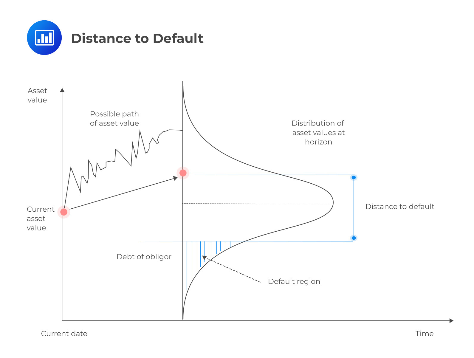
The Distance to Default

Distance to Default (DD) is a crucial concept within the Black-Scholes Option Pricing Model, especially in the context of credit risk analysis. It quantifies how close a company is to defaulting on its debt. DD measures the number of standard deviations by which the value of a firm’s assets exceeds its debt obligations. A higher DD implies a lower probability of default, indicating a healthier financial state. DD is a market-based risk measure, reflecting the volatility of the firm’s assets and their capacity to cover liabilities.

$$DD = \frac{\ln\left(\frac{A}{L}\right) + \left(\mu – \frac{\sigma_A^2}{2}\right)T}{\sigma_A \sqrt{T}}$$

Interpretation: A DD of 2.16 indicates that the firm’s asset value is approximately 2.16 standard deviations above the default point (where assets equal liabilities). This quantifies the firm’s ‘buffer’ against default, providing an insight into its creditworthiness.

Limitations of the Black-Scholes Merton Model in Credit Risk Management

• Complex market dynamics: The BSM Model, like other financial models, struggles to fully capture the complex socio-economic phenomena inherent in financial markets. The real-world financial market is influenced by a wide range of factors and interactions that are often too intricate and dynamic for any single model to accurately encompass.
• Simplifying assumptions: The BSM Model is based on several key assumptions, such as constant volatility, risk-free interest rates, and lognormal distribution of stock prices. While these assumptions are necessary for the model’s mathematical formulation, they may oversimplify actual market conditions. For example, volatility is known to fluctuate over time, and stock price movements do not always follow a lognormal distribution.
• Challenges in credit risk aggregation: When it comes to credit risk management, the BSM Model faces difficulties in aggregating and comparing credit risks across different business lines or financial institutions. This is due to the model’s focus on market-based risk factors, which may not fully align with the specificities of credit risk.
• Limited scope in financial contexts: The BSM Model is highly effective in options pricing and assessing certain market risks. However, its applicability may be limited in more complex financial scenarios, especially those involving non-standard financial instruments or unique market conditions.
• Dependence on historical data: The effectiveness of the BSM Model is contingent on the quality and relevance of historical market data. Market conditions and financial regulations that change over time can make historical data less predictive of future trends, potentially limiting the model’s accuracy and applicability.

The KMV Model

The KMV Model, developed by Moody’s KMV, represents a significant advancement in the field of credit risk assessment. This model is particularly renowned for its Expected Default Frequency (EDF™) approach, which offers a sophisticated way to gauge the likelihood of a borrower defaulting on their obligations.

Understanding the KMV Model

Focus on Asset Value and Volatility

The KMV Model’s central premise is the strong correlation between a firm’s likelihood of default and two key financial indicators: the market value of its assets and the volatility of these assets. This approach stems from the understanding that a firm’s asset value provides a snapshot of its financial health and capability to meet obligations, while asset volatility reflects the stability and predictability of these values over time.

• Market value of assets: This represents the current worth of all the firm’s assets if they were to be sold in the market. A high asset value relative to debt indicates a lower probability of default as the firm can theoretically liquidate assets to meet its obligations.
• Asset volatility: This measures the fluctuation in the value of the firm’s assets. Higher volatility indicates greater uncertainty and risk, implying a higher probability of default. This is because unpredictable changes in asset values can affect a firm’s ability to service debt.

System of Equations

The KMV Model utilizes a sophisticated mathematical framework derived from option pricing theory. The equations are based on the Black-Scholes option pricing model and Merton’s model for corporate debt pricing. These models treat a firm’s equity as a call option on its assets, with debt acting as the strike price. The model employs an iterative Newton-type algorithm to solve these equations. This process entails making an initial guess of the asset value and volatility, then refining these estimates through successive iterations until a stable solution is achieved. These calculations require inputs like the current market value of the firm’s equity, its volatility (derived from stock prices), the face value of debt, and the risk-free interest rate. The output is an estimated market value of assets (A) and their volatility (uA).

Probability of Default (PD)

The PD in the KMV model is a risk-neutral measure. This means it assumes investors are indifferent to risk, focusing solely on potential returns. This approach simplifies the calculation by not requiring subjective risk preferences. A higher PD suggests a greater chance that the firm will not meet its debt obligations, typically due to financial distress. This metric is vital for lenders and investors as it guides credit decisions and risk management strategies. PD is calculated by comparing the firm’s asset value to its debt level. If the asset value is likely to fall below the debt level (considering its volatility), the PD increases. This comparison essentially views equity as an option on the firm’s assets, with default occurring if the option falls ‘out of the money’ at debt maturity.

Expected Default Frequency (EDF™)

The EDF™ is a proprietary aspect of the KMV Model. This feature differentiates the model from others by how it maps the distance to default (DD) to a probability of default scale. Instead of relying on the normal distribution, the EDF™ approach utilizes a more complex methodology, enhancing the model’s accuracy in predicting defaults.

Implications and Usage

• Risk assessment: The KMV Model is widely used for assessing credit risk, especially in the context of corporate loans. It provides a more nuanced understanding of a firm’s financial stability and its ability to meet debt obligations.
• Investment and lending decisions: Financial institutions leverage the insights from the KMV Model to make informed decisions about lending to corporations and managing their credit portfolios.
• Regulatory compliance: The model’s sophisticated approach to estimating PD and its alignment with regulatory requirements makes it a valuable tool for complying with financial regulations, especially in risk-weighted asset calculations.

Black Scholes Model vs. KMV

Similarities

• Both models are grounded in option pricing theory.
• Each treats a firm’s equity as an option on its assets.
• They rely on the firm’s asset value and volatility for calculations.
• Both models are used to estimate the likelihood of a firm defaulting on its debt.
• Employed for risk assessment in financial and credit markets.
• Utilize a quantitative, mathematical approach for risk evaluation.

Key Differences

$$\small{\begin{array}{l|l|l}
\textbf{Feature} & \textbf{Black-Scholes Model} & \textbf{KMV Model} \\
\hline
\text{Default Probability Estimation} &
{\text{Typically uses a normal}\\\text{distribution for estimating PD}} &
{\text{Utilizes historical data to derive}\\\text{an empirical distribution of}\\\text{default frequencies for PD estimation}} \\
\hline
\text{Default Point Definition} &
{\text{The default point may not be}\\\text{explicitly defined}} &
{\text{Defines the default point as the sum}\\\text{of short-term debt and half of}\\\text{long-term debt for a more accurate}\\\text{approximation of loan obligations}} \\
\hline
\text{Empirical Data Usage} &
{\text{Less emphasis on historical data}\\\text{for PD calculation}} &
{\text{Heavily relies on historical data}\\\text{for determining PD}} \\
\hline
\text{Model Specificity} &
{\text{General application for assessing}\\\text{default risk}} &
{\text{Specifically tailored for credit risk}\\\text{assessment in financial firms}} \\
\hline
\text{Debt Structure} &
{\text{Does not specifically emphasize}\\\text{the structure of a firm’s debt}} &
{\text{Pays particular attention to both}\\\text{short-term and long-term debt in}\\\text{defining the default point}} \\
\hline
\text{Mapping of DD to PD} &
{\text{May not have a specific method}\\\text{for this mapping}} &
{\text{Uses a sophisticated approach to}\\\text{map Distance to Default to}\\\text{Probability of Default, considering}\\\text{firm-specific debt structures}} \end{array}}$$

The CreditMetrics Model

The CreditMetrics model is a sophisticated framework for evaluating credit risk, particularly distinguished by its comprehensive approach and detailed methodology.

Transition Probability Analysis

In assessing the probability of default, CreditMetrics stands out by its utilization of transition tables. These tables are instrumental in gauging the likelihood of changes in credit ratings over time, providing an analytical basis for predicting future creditworthiness. By comparing a company’s credit risk profile with those of similar companies that have defaulted, the model offers a relative perspective on default probability. This comparative analysis, grounded in real-world data, enhances the model’s ability to predict credit rating transitions accurately.

Mark-to-Market Approach

Diverging from the default mode models, CreditMetrics adopts a mark-to-market approach. This methodology involves the periodic revaluation of assets and liabilities based on prevailing market conditions, offering a more dynamic and realistic view of a company’s credit risk. By continuously adjusting to market fluctuations, the model ensures that credit risk assessments remain relevant and accurate, reflecting the current economic landscape.

Comprehensive Data Utilization

A key strength of CreditMetrics is its extensive use of comprehensive data, particularly the credit ratings of bond issuers and corresponding transition matrices. These matrices showcase the potential movement of an issuer’s credit rating across different levels, thereby capturing the fluid nature of credit risk. By integrating such detailed information, the model effectively tracks and predicts changes in creditworthiness over time.

Loan Value Distribution

CreditMetrics is adept at generating a distribution curve reflecting changes in a loan’s value over time. This analysis incorporates various factors, such as the present value of a bond, its coupon payments, prevailing risk-free interest rates, and the specific risk premium associated with each credit grade. Such a multifaceted approach provides a nuanced view of how a loan’s value might evolve, factoring in both market conditions and the bond’s inherent characteristics.

Methodology and Application

The model’s methodology is comprehensive, spanning a wide array of financial products. This breadth ensures systematic and holistic risk management, allowing for nuanced insights into diverse financial instruments. It is structured to offer portfolio risk measures that consider the interplay between individual assets and the overall portfolio, thereby facilitating strategic decision-making in portfolio management.

Three-Stage Risk Evaluation

CreditMetrics conducts its risk evaluation in three distinct stages: first, by profiling the exposure of various financial instruments; second, by estimating the volatility of these instruments due to potential credit rating changes; and finally, by aggregating these individual volatilities to calculate the total volatility of the portfolio. The final stage crucially accounts for correlations between different credit events, allowing for a consolidated view of portfolio risk.

Application and Usage

The CreditMetrics model is extensively used in various facets of financial risk management, offering a robust framework for credit risk analysis. Its applications include:

• Portfolio risk management: CreditMetrics is crucial for managing the risk of diverse financial portfolios. It assesses the potential changes in credit ratings of bonds and loans, enabling portfolio managers to understand and anticipate shifts in credit risk, thereby facilitating informed decision-making regarding asset allocation and risk mitigation strategies.
• Credit Risk analysis of financial instruments: The model finds extensive application in analyzing the credit risk of a broad range of financial instruments, including traditional loans, letters of credit, fixed income securities, and commercial contracts. Its comprehensive approach allows for a detailed evaluation of each instrument’s risk profile, considering factors like credit rating transitions and market dynamics.
• Assessment of market-driven products: In addition to traditional financial products, CreditMetrics is adept at analyzing market-driven instruments such as derivatives, swaps, and forward contracts. By integrating market-based data, the model offers a dynamic assessment of these instruments, reflecting the influence of market conditions on their credit risk.
• Regulatory compliance and reporting: CreditMetrics assists financial institutions in meeting regulatory requirements and enhancing transparency in credit risk reporting. Its structured methodology and standardized risk measures align with regulatory frameworks, making it a valuable tool for compliance and external supervision.
• Strategic financial planning: The model’s ability to project changes in credit risk and value over time is instrumental for strategic financial planning. Financial analysts and risk managers use CreditMetrics to forecast potential credit events and their impact on financial products, aiding in long-term financial planning and risk avoidance strategies.
• Dynamic valuation of assets and liabilities: Its mark-to-market approach allows for the continuous revaluation of assets and liabilities based on current market conditions. This dynamic valuation is essential for keeping credit risk assessments up-to-date and relevant in rapidly changing economic environments.

Criticism of the CreditMetrics Model

One of the primary criticisms of the CreditMetrics model is its reliance on the assumption that credit grades are homogeneous. This assumption can oversimplify the complex and often heterogeneous nature of credit risks associated with different financial instruments or entities. By treating different credit grades as essentially similar, the model might not fully capture the nuances and unique risk profiles inherent in each grade.

Another significant concern is related to the determination of the time horizon for the model’s projections and analyses. The model typically sets this horizon at one year, but it can be extended to much longer periods, such as up to 10 years. This flexibility, while advantageous in some respects, can also introduce uncertainties, especially given the inherent difficulty in accurately predicting long-term financial trends and behaviors.

Additionally, the model’s use of fixed interest rates for calculating recovery rates has raised concerns about its validity, particularly over longer time horizons. Interest rates can be highly volatile and subject to a wide array of influencing factors, including economic conditions, policy changes, and market dynamics. This volatility can significantly affect the model’s projections and risk assessments, potentially leading to less reliable or accurate outcomes.

The CreditRisk+ Model

The CreditRisk+ model, developed by Credit Suisse Financial Products in 1997, presents a unique approach in the landscape of credit risk modeling. Its development marked a significant divergence from traditional models like the KMV model, especially in its treatment of a firm’s capital structure.

Distinctive Features of the CreditRisk+ Model

• Independence from capital structure: Unlike the KMV model, the CreditRisk+ model does not rely on the capital structure of the company in assessing credit risk. This is a fundamental departure from conventional models that often link the likelihood of default to the financial leverage or other capital structure metrics of a company.
• Focus on bankruptcy and default events: The CreditRisk+ model distinguishes primarily between two credit events: bankruptcy and a general bad credit condition. This binary view simplifies the assessment process by focusing on the extremes of credit quality.
• Default frequency as a continuous variable: The model perceives the default frequency not as a discrete outcome but as a continuous random variable. This approach provides a more nuanced understanding of default probabilities, allowing for a more dynamic and responsive credit risk assessment.
• Utilization of the Poisson distribution: In the CreditRisk+ model, the probability of a borrower defaulting on obligations is seen as very small and independent of other credit events in the portfolio. The model employs the Poisson distribution to model this probability, suggesting an interesting relationship where the average default rate equates to its variance.

Implications and Usage

• Simplified data requirements: Due to its focus primarily on default events and its independence from a company’s capital structure, the CreditRisk+ model requires minimal data, making it an accessible and easy-to-use tool for financial institutions.
• Portfolio risk assessment: The model’s ability to combine individual credit event probabilities offers a comprehensive view of the entire credit portfolio’s risk profile. This holistic approach is crucial for financial institutions to understand and manage their aggregate credit risk exposure.
• Flexibility in risk modeling: The model’s unique approach to assessing default probabilities allows for flexibility and adaptability in various financial contexts. Its simplicity and focus on key credit events make it a versatile tool in the arsenal of credit risk management.

$$\small{
\begin{array}{l|l|l|l}
\textbf{Feature} & \textbf{CreditRisk+ Model} & \textbf{KMV Model} & \textbf{CreditMetrics Model} \\
\hline
\text{Developer} &
{\text{Credit Suisse Financial}\\\text{Products, 1997}} &
\text{Moody’s KMV} &
\text{J.P. Morgan, late 1990s} \\
\hline
\text{Focus} &
{\text{Bankruptcy and general bad}\\\text{credit conditions}} &
{\text{Firm’s asset value and}\\\text{capital structure}} &
\text{Transition of credit ratings and market data} \\
\hline
\text{Basis of Model} &
{\text{Poisson distribution for}\\\text{default events}} &
{\text{Option pricing theory}\\\text{(structural model)}} &
{\text{Mark-to-market}\\\text{(transitional model)}} \\
\hline
\text{Data Requirements} &
{\text{Minimal; mainly focused on}\\\text{default events}} &
{\text{Detailed data on capital}\\\text{structure and market value of}\\\text{equity}} &
{\text{Detailed data on credit ratings,}\\\text{market yields, and transition}\\\text{probabilities}} \\
\hline
\text{Capital Structure} &
{\text{No reliance on the capital}\\\text{structure of the company}} &
{\text{Relies heavily on the capital}\\\text{structure}} &
{\text{Does not directly use capital}\\\text{structure but requires market}\\\text{data that may be influenced by it}} \\
\hline
\text{Complexity} &
{\text{Lower complexity, easier to}\\\text{implement}} &
{\text{Higher complexity due to its}\\\text{reliance on market data and}\\\text{capital structure}} &
{\text{Moderate to high complexity,}\\\text{requires detailed market data}\\\text{and ratings transitions}} \\
\hline
\text{Main Application} &
{\text{Simplified risk assessment,}\\\text{particularly useful where data}\\\text{is scarce}} &
{\text{Detailed risk analysis for firms}\\\text{with accessible market data}} &
{\text{Risk quantification across a}\\\text{range of financial products,}\\\text{including non-marketable assets}} \\
\hline
\text{Risk Assessment} &
{\text{Focuses on binary outcomes}\\\text{(default/no default)}} &
{\text{Continuous assessment based}\\\text{on market fluctuations and}\\\text{asset values}} &
{\text{Based on rating transitions and}\\\text{market conditions, often over a}\\\text{set period}} \\
\hline
\text{Primary Use Case} &
{\text{General credit risk assessment}\\\text{with minimal data}} &
{\text{Sophisticated credit risk}\\\text{analysis for publicly traded}\\\text{companies}} &
{\text{Portfolio risk management and}\\\text{diversification strategies}}
\end{array}
}$$

Measuring the Financial Performance of Loans using the Risk-Adjusted Return on Capital (RAROC)

While credit risk assessment methodologies, including scoring and rating models, are typically validated through statistical performance measures, their practical application in day-to-day financial decision-making necessitates a different approach. Financial measures play a crucial role in evaluating loan performance and guiding decisions regarding loan acceptance or rejection. These measures assess the return of a loan in the context of its associated risk, integrating factors beyond analytical models such as regulatory requirements, fees, and the cost of capital. This integration bridges the gap between theoretical risk modeling and practical financial decision-making.

Risk-Adjusted Return on Capital (RAROC) has emerged as a pivotal metric within the financial industry, largely due to its ability to encapsulate efficient risk management’s contribution to an institution’s profitability. This measure is reflective of modern financial economies’ capability to identify, measure, and manage risk, and then incorporate it into strategic decision-making processes like risk mitigation.

RAROC operates by comparing the financial outcomes, namely income and profits, against the economic capital allocated for achieving these outcomes. This comparison is not static but varies depending on the specifics of the financial institution, product line, or individual loan being assessed.

In the realm of credit risk modeling, RAROC is employed to evaluate the performance of a loan by considering the revenues generated by the loan, net of expenses and expected losses. The economic capital in this context is defined as the capital at risk – essentially, the capital that a bank needs to reserve to safeguard itself against potential risk exposures in scenarios such as loan defaults.

The formula for RAROC, therefore, becomes a simple ratio:

$$\text{RAROC} = \frac{\text{Loan Revenues}}{\text{Capital at Risk}}$$

Numerator

In calculating RAROC, several key financial factors are taken into account in the numerator of the ratio. These include:

1. Spread Between Loan Rate and Bank’s Cost of Capital (s): This spread represents the difference between the interest rate charged on the loan and the bank’s own borrowing cost. It is a critical factor as it directly impacts the profitability of the loan.
2. Fees Attributable to the Loan (f): Loan-related fees contribute to the revenue generated from the loan. These can include origination fees, processing fees, or any other charges directly associated with the loan issuance.

• Expected Loan Losses (l): This component reflects the anticipated losses on the loan. It’s a provision based on historical data and predictive models, accounting for the possibility that the loan may not be fully repaid.

1. Operating Costs (c): Operating costs are the expenses incurred in managing and servicing the loan. These costs can vary depending on the loan’s complexity, duration, and required administrative support.
2. Taxation (x): Taxes play a significant role in the overall profitability of a loan. The impact of taxation must be considered to understand the net revenue from the loan.

Using these components, the expected revenues from a loan can be formulated as follows:

$$\text{Loan Revenues} = (s + f – l – c) \cdot (1 – x)$$

Denominator

The Market-Based Approach

One way to define capital at risk for the calculation of RAROC is to use the change in the value of the loan during the period under consideration (usually 1 year), due to changes in interest rates. For this purpose, the duration of the loan can be used as a measure of the loan’s value sensitivity to interest rate changes. Duration, in this context, is not merely a measure of time but an indicator of how much the value of the loan might decrease if interest rates were to rise. Specifically, for a loan with a principal amount (L), a given duration (D), and a fixed interest rate (i), the change in the loan’s value (ΔL) relative to an incremental change in interest rates \((Δi)\) is approximated by the formula:

$$\Delta L = -LD \cdot \frac{\Delta i}{1 + i}$$

For example, consider a loan with a principal of €1,000,000, a duration of 4 years, and an interest rate of 12%. If the interest rates increase by 2% (or 0.02), the estimated reduction in the loan’s value would be around €71,429. This figure represents the capital that the bank risks losing due to the interest rate increase and is therefore the ‘capital at risk’ in the RAROC formula.

Moreover, if we factor in additional revenues such as loan servicing fees—at, say, 0.1%—and the spread between the loan’s interest rate and the bank’s cost of funds—let’s say 0.3%—the annual revenue from the loan (excluding expenses and expected losses) becomes €4,000 (i.e., 0.4% × 1,000,000). With this revenue and the calculated capital at dvcsdsdssdisk, the RAROC for this loan would be:

$$\text{RAROC} = \frac{4,000}{71,429} \approx 5.6\%$$

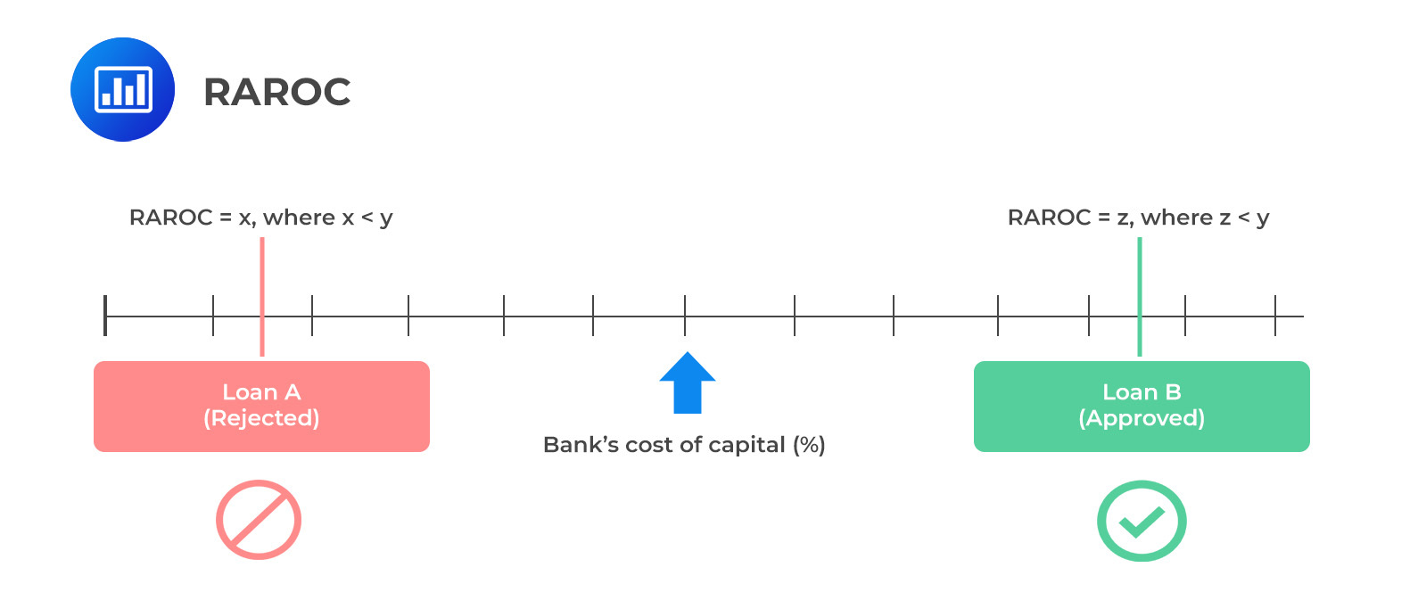
This RAROC value is critical in decision-making: if it surpasses the bank’s own cost of capital, the loan is adjudged profitable. This profitability threshold is bank-specific, reflecting each institution’s risk appetite and capital cost structure. The RAROC measure, therefore, not only guides banks in pricing loans and setting interest rates but also serves as a strategic tool for managing their loan portfolios in alignment with broader financial goals and market conditions.

The Unexpected Loan Loss

In the evaluation of a loan using Risk-Adjusted Return on Capital (RAROC), particularly when models for predicting defaults are employed, an alternative method for determining the denominator of the RAROC ratio is the calculation of unexpected loan loss. This approach provides a more nuanced view of the potential risk associated with a loan by factoring in unforeseen events that could lead to default, beyond what traditional analyses might capture.

The formula for calculating unexpected loan loss is:

$$\text{Unexpected loan loss} = \alpha \cdot LGD \cdot EAD$$

In this equation, LGD represents the ‘Loss Given Default,’ which is the percentage of the loan that will not be recovered in the event of default. EAD, or ‘Exposure at Default,’ signifies the total value at risk when the borrower defaults. The variable α (alpha) stands as a risk multiplier that reflects the unexpected default rate, which is not anticipated within the normal course of business.

The value of α is derived from the historical distribution of default rates for loans that are similar to the one being analyzed. For example, if historical default rates follow a normal distribution, α could be set at a value corresponding to a high confidence level, such as 2.6 times the standard deviation (s) of those rates for a 99.5% confidence level. This multiplier provides a buffer to accommodate the uncertainty and variability in default rates.

However, it is important to note that loan loss distributions tend to deviate from the normal distribution, often being skewed due to the nature of credit events. Therefore, a higher coefficient for the standard deviation—possibly in the range of 5 to 6—is sometimes used. This adjustment accounts for the skewness and ensures that the capital at risk is adequately estimated to cover potential unexpected losses.

This alternative method, incorporating unexpected loan loss into RAROC calculations, is particularly useful for financial institutions as it aligns the risk management framework with real-world scenarios where defaults can often be unpredictable and unevenly distributed.

Practice Question

During a training session on advanced credit risk modeling techniques, an instructor is explaining the Black-Scholes Option Pricing Model to a group of credit analysts. The focus shifts to the limitations of the model in the context of credit risk analysis. One of the analysts asks about the main drawback of using the Black-Scholes model for assessing credit risk. Which of the following best describes a significant limitation of the Black-Scholes model in this context?

A. It overemphasizes the role of operational risks in a firm’s creditworthiness. B. It depends heavily on market data and assumptions about asset volatility. C. It primarily focuses on the firm’s historical performance. D. It disregards market data and relies solely on accounting ratios.

The correct answer is B.

The significant limitation of the Black-Scholes Option Pricing Model in credit risk analysis is that it depends heavily on market data and assumptions about asset volatility. The model requires accurate and current market values of the firm’s assets and assumes that the volatility of these assets remains constant over time. This reliance on market data and the assumption of constant volatility can lead to inaccuracies in credit risk assessment, especially during periods of market instability or for firms with volatile asset values.

A is incorrect because the Black-Scholes model does not primarily focus on operational risks in assessing a firm’s creditworthiness. Its main concern is the market value and volatility of a firm’s assets in relation to its debt obligations.

C is incorrect because the model does not primarily focus on a firm’s historical performance. Instead, it uses current market data to estimate the probability of default and other credit risk metrics.

D is incorrect because the Black-Scholes model does not disregard market data; in fact, it heavily relies on market data for its calculations. It does not solely depend on accounting ratios for credit risk assessment.

Things to Remember

• When using the Black-Scholes model in credit risk analysis, it’s important to be aware of the potential for inaccuracies due to market volatility and the limitations of the model’s assumptions.
• Analysts should consider supplementing the Black-Scholes model with other methods of credit risk assessment that may account for factors such as historical performance, operational risks, and qualitative assessments.
• The model’s effectiveness can vary across different types of firms and market conditions, so its use should be context-specific and part of a broader toolkit for credit risk analysis.