


Assessing the Quality of Risk Measures
After completing this reading, you should be able to: Describe the ways through... Read More

After completing this reading, you should be able to:
The 2007-2009 financial crisis exposed flaws and informed the establishment of solvency and liquidity regulations. Moreover, it exposed the market practice and product structures that were not able to withstand stressful periods. As a response to these flaws, global regulators came up with more strict regulations and supervision.
The Financial Stability Forum was a body that frequently conducted research. Later, it transformed into the Financial Stability Board (FSB). FSB consisted of representatives from different sectors, such as central banks, prudential regulators, and finance ministries. FSB became the body that approves international standards. However, after the crisis, FSB concentrated on other issues. Note that other institutions, such as the Basel Committee, retained their independence and authority.
The Global Financial Crisis of 2007-2008 proved that the minimum capital charges under the market risk amendment were not sufficient to address trading-book risks. This was evident in that, during the crisis, the market prices of financial assets fell sharply, hedging strategies failed, and there was doubt about securitizations.
Consequently, the Basel Committee reacted by introducing three main changes by the end of 2011:
Numerous banks calculated capital based on the market risk amendment using historical simulation. Remember that the market risk amendment involved the calculation of 1-day VaR by drawing the daily changes from the recent history and then scaling the same by \(\sqrt { 10 } \). However, VaR slowly decreases during the low volatility periods because the historical observations were small in value. Moreover, during high volatility periods (such as in 2007 for the majority of assets), historical VaR was slow to reflect since analysts took historical observations from low volatility periods.
Consequently, the Basel Committee recommended the stressed VaR. Instead of drawing daily observations from the recent historical time, a bank was advised to pick a one-year (250-day period) period from the last seven years that shows stress to its current portfolio. The VaR for this period would be intuitively high and unchanged unless the period of low volatility remains for seven years.
The stressed VaR expanded the traditional VaR measure to get:
$$ \text {M}{ \text {R}}_{ 2.5 }=\text {max} \left( \text {Va}{ \text {R} }_{ \text {t}-1 },{ \text {m} } \times \text{Va}{\text {R} }_{ \text {avg} } \right) +\text {max}\left( \text {SVa}{ \text{R} }_{ \text{t}-1 },{ \text{m} }_{ \text{s} }\times \text{S}{ \text{VaR} }_{ \text{avg} } \right) $$
Where:
\(\text {Va}{ \text {R} }_{ \text {t}-1 }\) and \(\text{Va}{\text {R} }_{ \text {avg} }\) are traditional 10-day, 99% VaR computed from the previous day and average from the 60 most recent days respectively.
\(\text {SVa}{ \text {R} }_{ \text {t}-1 }\) and \(\text {SVa}{ \text {R} }_{ \text {avg} }\) are computed for equivalent times as above but from the most stressful period in the past seven years.
\({ \text{m} }\) and \({ \text{m} }_{ \text{s} }\) are the multipliers, which according to the 1996 amendment, should, at least, be equal to 3.
It is worth noting that if the multipliers are equal for both the traditional VaR and stressed VaR, then \(\text {M}{ \text {R}}_{ 2.5 }\) must, at least, be twice MR under the 1996 amendment.
Incremental Risk Charge (IRC) was first introduced in 2005 as a result of regulation on arbitrage opportunities between the banking and trading book. Besides, regulators introduced IRC as a result of the Global Financial crisis.
Specific risk charges were meant to cover the default risk and some idiosyncratic risks. However, by the early 2000s, banks realized that even in the presence of specific risk charges, the majority of banking-book exposure needed lesser capital requirements in the trading book than in the banking book. Consequently, banks categorized illiquid assets with predisposing default risk in the trading book.
As a response to this drawback, the Basel Committee proposed an addition of incremental default risk charge (IDRC), which had two methods of calculation:
Towards the end of the crisis, the committee realized that portfolio losses were mainly associated with credit resulting from changes in ratings, credit spreads, or liquidity, not defaults. Therefore, the IRC was an amendment to include the changes in ratings in that the \({99.9}^{\text{th}}\) percentile was maintained, but the banks were required to approximate losses due to rating downgrades. The credit quality of a portfolio was approximately held constant by virtue that a position replaces the downgraded position of defaulting one with the same pre-downgraded rating. The replacement period differs across the positions based on the liquidity level but not less than three months.
Gordy’s (2003) model in Basel II assumes that the correlation parameter is constant across the obligors (but not across assets) over time. This assumption is only relevant to the debt instruments portfolio so that the banking-book capital can be determined effectively. However, the assumption does not apply to correlation book securitizations and derivatives written on securitizations.
The correlation book puts a portfolio in a special purpose vehicle and generates tranche liabilities that differ in seniority and, therefore, in their credit losses. Conventionally, correlations change over time and, as such, in this context, change the value of the trances. For instance, the AAA-rated tranches had a low default rate in the pre-crisis period, but the PD changed in times of crisis, and thus their prices fell.
To address this issue, the Basel Committee substituted the incremental risk charge (IRC) and the specific risk charge with the comprehensive risk (CR) charge for the correlation book. Under this new dimension, banks may use a standardized approach that only depends on the ratings of the instruments. The ratings were as shown below:
$$ \begin{array}{l|c|c|c|c|c} {} & \textbf{AAA,AA} & \textbf{A} & \textbf{BBB} & \textbf{BB} & \textbf{Less than BB, unrated} \\ \hline \text{Securitizations} & {1.6\%} & {4\%} & {8\%} & {28\%} & {100\%} \\ \hline \text{Re-Securitizations} & {3.2\%} & {8\%} & {18\%} & {52\%} & {100\%} \\ \end{array} $$
Note that the percentages are not the risk weights but rather the capital as a fraction of exposure. Moreover, since re-securitizations are more valuable to correlation changes and hence higher capital requirements, the tranches that fall into rating BB and below attract more capital charges because they are prone to losses.
The Basel Committee proposed that banks could also use the internal model to compute the CR charge only after approval from the supervisors. The model-based charge may not be less than the fraction under the standardized approach, and it is more complicated than the standardized approach.
Apart from the weaknesses of the Basel II stated earlier, the global financial crisis unraveled more flaws in the Basel II accord:
To address the above flaws, BCBS published proposals in December 2010 as “Basel III: International framework for liquidity risk measurement standards and monitoring” and in June 2011 as “Basel III: A global regulatory framework for more resilient banks and banking systems.” The components of Basel III are discussed below.
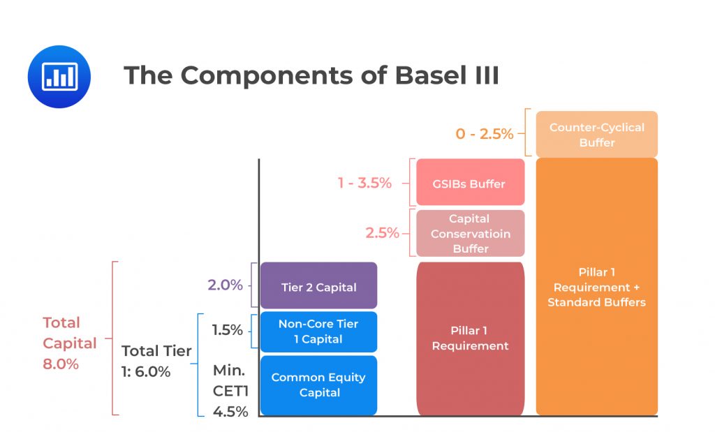 Basel III Capital Definition
The Basel III removed Tier 3 Capital and divided Tier 1 capital into:
Moreover, the minimum capital requirements were also amended as follows:
Moreover, the constituents of each capital category were changed:
Goodwill and other intangibles, deferred tax assets, and any other shortfall reserves based on IRB expected losses are subtracted from the Tier 1 Equity Capital.
There were the required subtractions such as:
The general feature of the Basel III accord is that compared to Basel II, its capital requirements were higher. This was because the minimum ratios were increased and allowable capital restricted.
Before the Basel III accord, the minimum capital ratios were expressed by the Basel Committee as the percentage of RWA. However, in the post-crisis period, many observers noted that this had underestimated the risks faced by banks and hence overleveraged. Although flaws in the calculation of RWA were addressed, its future errors were imminent. Moreover, market participants concentrated on simple ratios of equity to unweighted assets as they determined the soundness of banking organizations, making the risk-weighted ratio value subject of discussions.
Reacting to the above flaws, the Basel Committee proposed a “simple” leverage ratio capital requirement as a supplement to the risk-based requirements. This simple leverage capital ratio requires banking organizations to maintain a ratio of Core Tier 1 Capital to Leverage Exposure of at least 3%.
Note that the leverage exposure incorporated both the on-balance-sheet and off-balance-sheet assets. The handling of off-balance-sheet assets by the committee was somewhat different from IFRS and GAAP accounting principles. Even then, it was much more detailed to allow comparison across different countries.
The Financial Stability Board (FSB), in cooperation with the International Association of Insurance Supervisors (IAIS), publishes the list of the globally systematically important banks (G-SIBs) and globally systematically significant insurers (G-SII). In some cases, some nations assign some banks to be G-SIBs.
G-SIBS, G-SIIs, and other firms are classified as systematically important financial institutions (SIFIs). For a firm to qualify as SIFI, FSB determines the size, complexity, interconnectedness, and other factors of the firm. A firm is regarded as SIFI if its failure or distress is amplified to the whole financial system or the real economy. For instance, the whole financial market and its counterparties felt the failure of Lehman Brothers.
SIFIs are often regarded as “too big to fail.” Still, the main objective of this is to lower the probability of it failing and make it not disrupt the real economy of the financial system in case it fails. Moreover, in the event of failure, the shareholders will be eliminated, and creditors will experience losses. However, a SIFI should continue operating and should recapitalize without government assistance. Lastly, SIFIs are subject to a wide range of supervision and regulation.
By early 2019, Basel had specified the requirements for capital above the minimum fractions of RWA. These include:
The rationale in the case of countercyclical capital buffer (CCyB) is similar to the US regulation Prompt Corrective Action (PCA) of 1991. This regulation stipulates that a bank with ratios nearing the minimums should be subjected to more stringent supervision in a bid to return it to a well-capitalized status. The restrictions induced by the committee were restrictions on dividend and bonus payments and planned to restore the ratios.
The rationales in the case of CCyB were to give an instrument for macroprudential control of overheating and address the cost of capital. Overheating, in this case, implies that a higher capital requirement limits the credit supply by the banks and thus causing overheating in the credit market, lowering the maximum point of the credit cycle, and thus reducing the frequency and severity of the financial crisis. The demerit of this rationale is that the calculation of CCyB for a bank with international activities is sophisticated because CCyB differs across the nations. In addition, a bank with international operations might be required to give a combined average of CCyB as a weighted average of the requirements in each nation.
In the case of cost of capital, the rationale supposes that the cost of a bank’s increase in its capital ratio is less in good times than in bad times. For this reason, financial stability can be increased by achieving a lower cost by increasing CCyB during good times and lowering it during bad times.
For the case of G-SIB, the rationale is similar to that of CCB, only that it recognizes the impact of the distress at G-SIB on society. Therefore, higher buffers are stated to lower the likelihood of further failure.
The BCBS finalized the reforms in December, including the revisions of the previous accord. These revisions include:
Additionally, the output floor was introduced. This made sure that the capital calculations under the ratings-based and other models are capped at not less than 72.5% of the standardized approach.
The Basel III accord proposed two methods of calculating CVA risk:
A standardized approach replaces the Basel II approach to calculating operational risk. The main characteristics include the business indicator (BI) and the business indicator component (BIC). BIC is equal to BI multiplied by the internal loss multiplier (ILM). ILM is the scaling factor based on historical losses. The business indicator is given by:
$$ \text{BI}=\text{ILDC+SC+FC} $$
Where:
\( \begin{align*} \text{ILDC} & = \text{min}[\text{Abs}\left(\text{Interest Income–Interest Expense}\right), \ 2.25\% \\ & \times \text{Income Earnung Assets+Divident Income]} \end{align*} \)
\( \begin{align*} \text{SC } & = \text{max}[\text{Other Operating Income, Other Operating Expense} \\ & + \text{max}(\text{Fee Income, Fee Expense)]} \end{align*} \)
\(\text{FC} = \text{Abs}\left(\text{Net P&L Trading Book} \right) +\text{Abs}\left(\text{Net P&L Banking Book}\right) \)
The internal loss multiplier (ILM) is defined as:
$$ \text{ILM}=\text{ln } \left[ \text{exp}\left( 1 \right) -1+{ \left( \cfrac { \text{LC} }{ \text{BIC} } \right) }^{ 0.8 } \right] $$
The BIC is defined as follows:
Financial institutions that seem to be solvent can be exposed to running due to withdrawal by the depositors and counterparties. The withdrawals, in such instances, exceed what assets can cover. Regardless of the cause of the run, authorities desire to find a solution without involving the government.
Basel III addressed the liquidity risk by providing two requirements:
The LCR is structured to give the banks and authorities a month to address the crisis by selling liquid assets. The concept behind LCR is that if a bank has liquid assets (assets that can be sold quickly and are reasonably priced) whose sum value exceeds what it needs to cover liquidity requirements, it can sell its assets in an attempt to redeem itself.
The LCR requirement is defined as:
$$ \text{LCR}=\cfrac {\text{ High quality liquid assets}\left( \text{HQLA} \right) }{ \text{Net cash outflows in a 30 day period} } >1 $$
The HQLA is determined by classifying assets and applying haircuts based on the likely availability of buyers at prices near normal-times values. For instance, HQLA with no haircuts refers to the deposits at the central banks, government-issued securities (with 0 risk weight), and equity, which has 50% haircuts. Individual mortgage loans are excluded from the HQLA category.
The NSFR utilizes a one-year time horizon and focuses on what remains after the stressful period rather than what can be sold. The NSFR requirement is defined as:
$$ \text{NSFR}=\cfrac { \text{Available amount of stable funding} }{ \text{Required amount of stable funding} } >1 $$
The available amount of stable funding is equivalent to the product of the amount in several categories and the available stable funding (ASF) factors (which can be thought of as haircuts). Note, however, that the categories are different from that of LCR. The required amount of stable funding is calculated by multiplying the amounts in each category of assets by the required stable funding (RSF) factor. The RSF for liquid assets is higher than that of illiquid assets.
The Bank of Afrika has liabilities of USD 800 million of stable retail deposits with not more than six months remaining to maturity. The bank has a 4-month certificate of deposit of USD 400 million, with each quarter maturing each month. The bank has USD 300 of 8-year senior bonds with none maturing in the next year and USD 200 common equity. The several ASF factors for these liabilities are 90%, 0%, and 100%.
On the assets side of the bank, it has USD 200 of valued cash, USD 200 debt of its sovereign, USD 200 of corporate debt securities rated BBB in the trading account, and USD 800 of loans to business with eight months remaining maturity. The respective RSF factors are 0%, 10%, 50%, and 80%.
What is the value of the net stable funding ratio (NSFR)?
The NSFR is defined as:
$$ \begin{align*} \text{NSFR} & =\cfrac { \text{Available amount of stable funding} }{ \text{Required amount of stable funding} } >1 \\ & =\cfrac {0.90 \times 800+0\% \times 400+100\% \times \left( 300+200 \right) }{ 0\% \times 200+10\% \times 200+50\% \times 200+80\% \times 800 } > 1 \\ & =\cfrac { 720+0+500 }{ 0+20+100+640 } =1.645 \end{align*} $$
So the bank will comply with the NFSR.
Banks are required to compute the credit adjustment (CVA) for each derivative counterparty. The CVA is defined as the difference between the value of the risk-free portfolio (of that particular counterparty) and the value of the actual portfolio. Intuitively, CVA rises with the counterparty’s credit spread. Also, CVA is affected by the portfolio market value variation, which in turn affects the profit.
Banks are still prone to failure even after all the Basel Accords and other reforms. To reduce the effects of such failures, FSB agreed in 2014 that the national resolution regimes for G-SIBs would possess 12 attributes. In addition, FSB resolved that each G-SIB should have the sufficient total loss-absorbing capacity (TLAC) to give it the ability to recapitalize itself.
Recapitalization might be achieved by causing convertible bonds to become equity. Alternatively, recapitalization can be achieved by bail-in. That is, a specific wholesale debt liability is written down or converted to equity where the terms of conversion are spelled out into the indentured convertible bonds, which need conversion when the banks seem to be solvent. The bail-ins are overseen by national law, and the authority determines its structure after taking control of the bank.
Contingent convertibles (CoCos) are debt instruments that can convert a bond into equity or stock once a specific strike price is breached. Convertible bonds are issued by a firm that desires to avoid dilution of issuing equity prior to the improvement of its performance. At the holder’s option, convertible bonds can be converted into equity when a firm’s share price rises above the limit written in the indenture.
Contingent convertible bonds (CosCos) cause a bank’s equity to rise when distress occurs, as shown by triggers written into the indenture and not the option of the option. With CosCos, equity increases due to conversion to equity or when its value is written down.
Some of the varied triggers include when the ratio of Core Tier 1 Capital to RWA falls below the limit or when a bank’s main regulator declares the nonviability of the CosCos. CosCos can be incorporated in Additional Tier 1 if the limit set is more than or equal to 5.125% or other included in Tier 2.
Cocos are debt instruments when issued, but the holders receive less or no returns as compared to equity holders when a bank performs well. On the other hand, holders bear losses that are almost similar to the equity holders when a bank fails and, therefore, seem expensive to the banks when they issue.
However, the accounting advantage of the CosCos lies in the fact that they are not put in the equity account until they are converted, and, therefore, a bank can report high profits on equity.
Some countries required G-SIBS to prepare a detailed resolution framework that expounds on how to capitalize themselves when in distress, how they would fund themselves, and how they would continue operating as a going concern even when subsidiaries fail, among other critical issues.
The Basel Accord (I, II, III) achieved a significant level of uniformity across countries, but there are some key differences. For instance, there exist differences in accounting standards, bankruptcy laws, and regulations. Notably, even with an existing agreement in Basel, some jurisdictions apply more stringent regulations than others.
Even though the participating countries are not required to impose lenient domestic laws and regulations on globally active banks, they may impose requirements that are relatively different but higher than the Basel Accord. This is beneficial for the Basel negotiations because it grants freedom to those countries that want stringent standards that are applied domestically.
Basel expects that on top of its minimum standards, each country has the mandate to oversee banks and take appropriate actions to ensure that they have sufficient capital and liquidity and efficient risk management and governance. For instance, in the US, supervised stress tests based on supervisory models and scenarios are conducted in a bid to make sure that banks have a capital and liquidity planning process, risk management, and sufficient buffers to allow compliance with minimum capital and liquidity standards, even when they (banks) are undergoing a stressful period.
The reforms include:
Practice Question
Which of the following statements is correct about the stressed VaR in Basel 2.5?
A. Stressed VaR is calculated by multiplying 1-day VaR from the recent daily variation in values by \sqrt{10}.
B. Stressed VaR is drawn from one year from the most recent seven years that exhibited stress in its current portfolio.
C. Stressed VaR is drawn from one year from the most recent ten years that exhibited stress in its current portfolio.
D. None of the above.
The correct answer is: B).
A bank was required to identify a one-year (that is, 250 trading days) period from the latest seven years that was most stressful for its current portfolios.
Option A is incorrect: This was the method of calculating the market risk amendment using the historical simulation in the Basel I accord.
Option C is incorrect: Basel 2.5 required banks to identify one year from the latest seven years (not ten years) that was most stressful for its current portfolios.
Offered by AnalystPrep


