Digital Resilience and Financial Stabi ...
After completing this reading, you should be able to: Describe characteristics of cyber... Read More
After completing this reading, you should be able to:
Extreme value is either a very small or a very large value in a probability distribution. In FRM parlance, an extreme value is one that has a low probability of occurrence but potentially disastrous (catastrophic) effects if it does happen. In other words, the occurrence of extreme events is very rare but can prove very costly in financial terms.
Some of the events that can result in extreme values include:
The main challenge posed by extreme values is that there are only a few observations from which a credible, reliable analytical model can be built. In fact, there are some extreme values that have never occurred, but whose occurrence in the future can never be ruled out. Trying to model such events can be quite an uphill task.
Researchers tackle the challenge by assuming a certain distribution. However, choosing a distribution arbitrarily is ill-suited to handle extremes. This is because the distribution will tend to accommodate the more central observations because there are so many of them, rather than the extreme observations, which are much sparser.
Extreme value theory (EVT) is a branch of applied statistics developed to address study and predict the probabilities of extreme outcomes. It differs from “central tendency” statistics where we seek to dissect probabilities of relatively more common events, making use of the central limit theorem. Extreme value theory is not governed by the central limit theorem because it deals with the tail region of the relevant distribution. Studies on extreme value make use of what theory has to offer.
There are several extreme value theorems that seek to estimate the parameters used to describe extreme movements. One such theorem is the Fisher–Tippett–Gnedenko theorem, also known as the Fisher–Tippett theorem. According to this theorem, as the sample size n gets large, the distribution of extremes denoted \(\text M_{\text n}\) converges at the generalized extreme value (GEV) distribution.
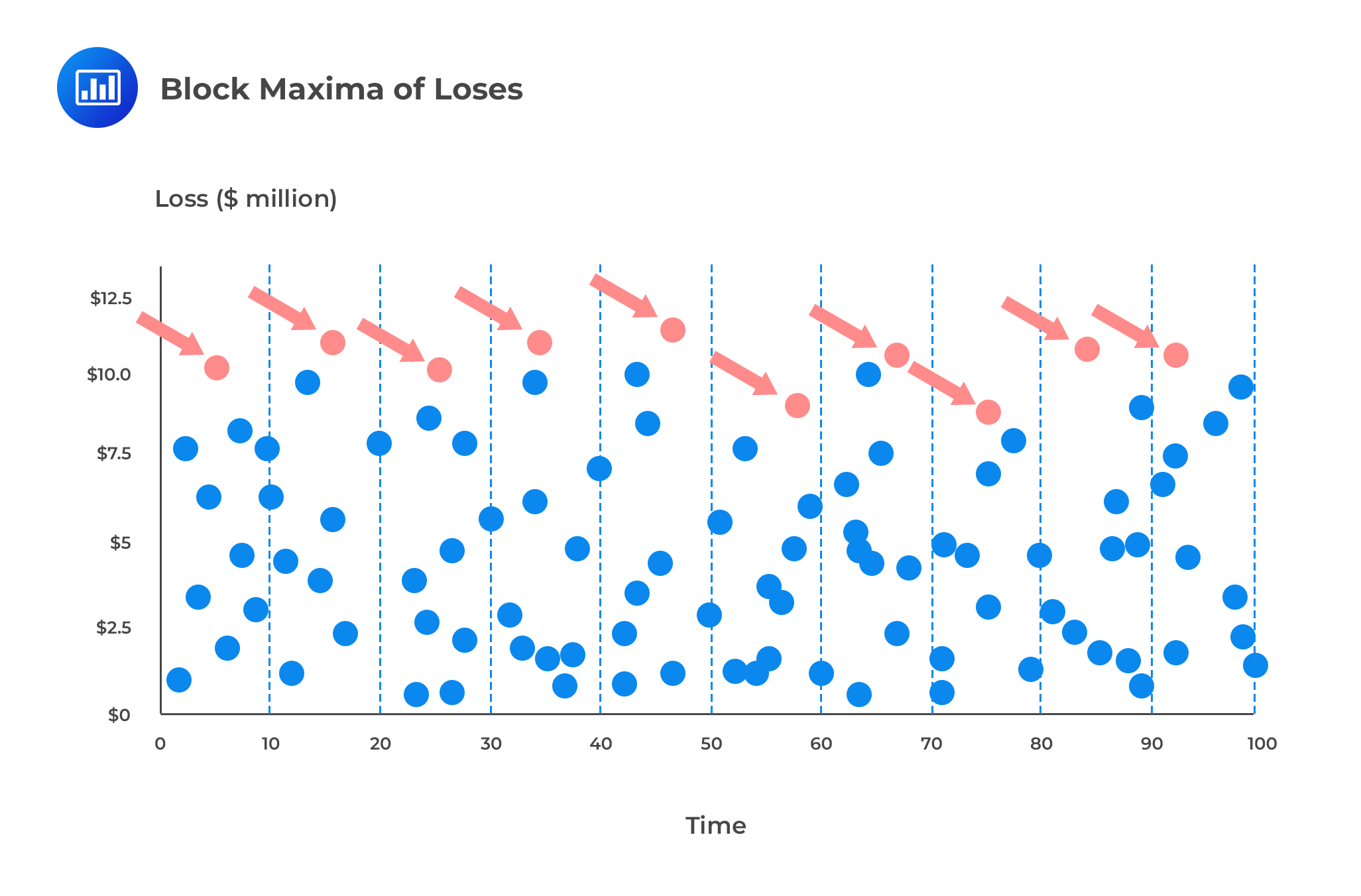
The generalized extreme value distribution is used to model the smallest or largest value among a large set of independent, identically distributed random values that represent observations. For example, let’s say we wish to assess the efficiency of a machine after detecting a series of products of uneven size. Assume we have organized items in batches of 100. If we record the size of the largest item in each batch, the resulting data are known as block maxima. If we record the size of the smallest item in each batch, we will end up with block minima. We can use the generalized extreme value distribution as a model for those block maxima or minima.
In risk management, we can segregate losses recorded over equal time intervals, say, 10 day periods, and record the largest loss in each interval. If we record the largest loss in each interval, we will end up with block maxima. We could then use the GEV distribution to estimate probabilities of extreme losses based on the block maxima (see figure below).
 The probability density function for the generalized extreme value distribution with location parameter \(\mu\), scale parameter \(\sigma\), and shape parameter \(\xi \) is:
$$ \text F(\xi ,\mu,\sigma)=\text{exp} \left[ – \left( 1+\xi × \cfrac {\text x-\mu}{\sigma} \right)^{-\frac {1}{\xi}} \right] \text{ if } \xi \neq 0 $$
And,
$$ \text F(\xi ,\mu,\sigma)=\text{exp}\left[-\text{exp} \left( -\cfrac{\text x-\mu}{\sigma} \right) \right] \text{ if } \xi = 0 $$
For these formulas, the following restriction holds:
$$ \left( 1+\xi × \cfrac {\text x-\mu}{\sigma} \right) > 0 $$
As noted, the parameter \(\xi\) indicates the shape (heaviness) of the tail of the limiting distribution.
There are three general cases of the GEV distribution:
\(\xi > 0\): The GEV becomes a Fréchet distribution, and the tails are “heavy,” as is the case for the t-distribution and Pareto distributions. This case is particularly relevant for financial returns, most of which are heavy-tailed, and we often find that estimates of \(\xi\) for financial return data are positive but less than 0.35.
\(\xi=0\): The GEV becomes the Gumbel distribution, and the tails are “light,” as is the case for the normal and lognormal distributions.
\(\xi < 0\): The GEV becomes the Weibull distribution, and the tails are “lighter” than a normal distribution.
In risk management, we focus on cases 1 and 2. Distributions where \(\xi<0\) do not often appear in financial models.
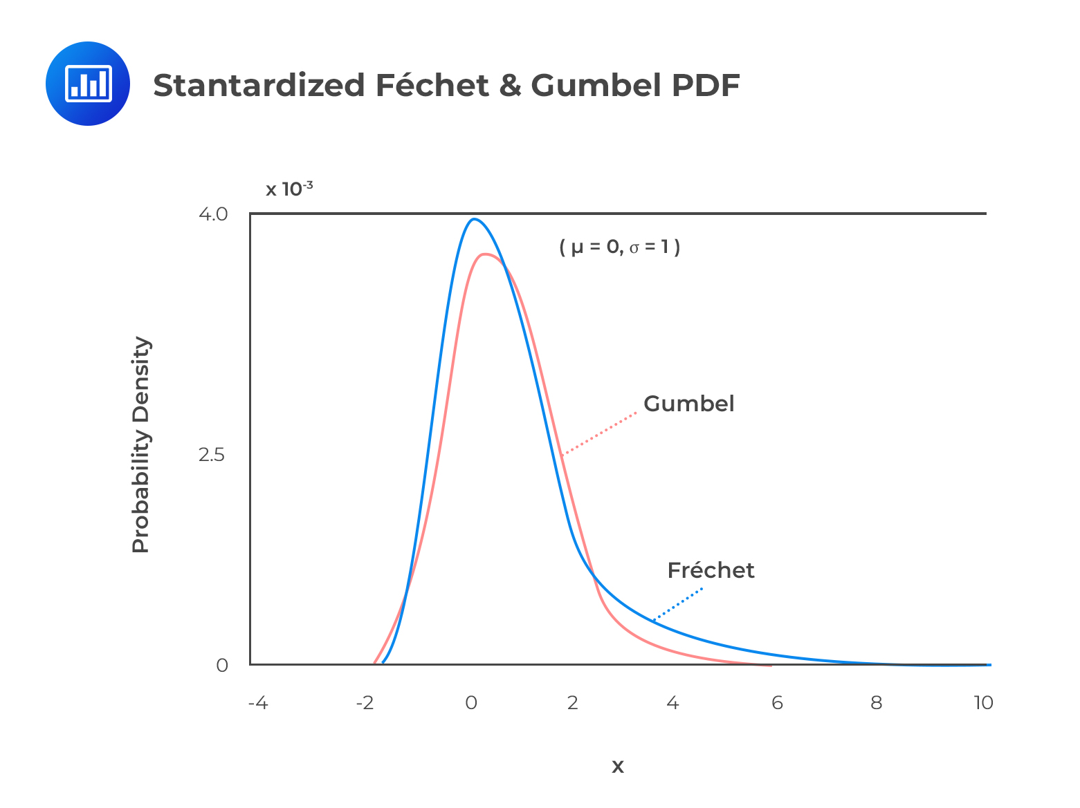
The figure below illustrates the standardized \((\mu=0,\sigma=1)\) Fréchet and Gumbel probability density functions.
 From the figure, we single out two main points:
We can obtain the quantiles associated with the GEV distribution as follows:
$$ \begin{align*} \text x & =\mu-\cfrac {\sigma}{\xi} \left[1-(-\text{ln(p)})^{-\xi} \right] \quad \quad \text{ (Fréchet,} \xi >0) \\ \text x & =\mu-\sigma \text{ ln}\left[-\text{ln(p)}\right] \quad \quad (\text{Gumbel}, \xi=0) \\ \end{align*} $$
where p is the chosen cumulative probability, and x is the observed value associated with the pth quantile.
For the standardized Gumbel, determine the 5% quantile, 95% quantile, and the 99% quantile.
First recall that for the standardized Gumbel, \(\mu=0,\sigma=1\)
$$ \text x=\mu-\sigma \text{ln} \left[-\text{ln(p)} \right] $$
$$ \begin{align*} & \text{The }5\% \text{ quantile is}: 0-(1)\text{ln}[-\text{ln}(0.05) ]=-1.0972 \\ & \text{The }95\% \text{ quantile is}: 0-(1)\text{ln}[-\text{ln}(0.95) ]=2.9702 \\ & \text{The }99\% \text{ quantile is}: 0-(1)\text{ln}[-\text{ln}(0.99) ]=4.6001 \\ \end{align*} $$
For the standardized Fréchet with \(\xi=0.3\), determine the 5% quantile, 95% quantile, and the 99% quantile.
$$ \text x=\mu-\cfrac {\sigma}{\xi} [1-(-\text{ln(p)})^{-\xi} ] $$
$$ \begin{align*} & \text{The }5\% \text{ quantile is}: -\cfrac {1}{0.3}[1—(-\text{ln}(0.05))^{-0.3}]=-0.9348 \\ & \text{The }95\% \text{ quantile is}: -\cfrac {1}{0.3}[1—(-\text{ln}(0.95))^{-0.3}]=4.7924 \\ & \text{The }99\% \text{ quantile is}: -\cfrac {1}{0.3}[1—(-\text{ln}(0.99))^{-0.3}]=9.9169 \\ \end{align*} $$
It is important to interpret these quantiles correctly. The above probabilities refer to the probabilities associated with the extreme loss distribution, and have nothing to do with the ‘parent’ loss distribution from which the extreme losses are drawn.
The 5th percentile, for example, is the cut-off point between the lowest 5% of extreme (high) losses and the highest 95% of extreme (high) losses; it is not the 5th percentile point of the parent distribution. The 5th percentile of the extreme loss distribution is, therefore on the left-hand side of the distribution of extreme losses (because it is a small extreme loss), but on the right-hand tail of the original loss distribution (because it is an extreme loss).
The VaR at \(\alpha\) level of confidence is given by:
$$ \begin{align*} \text {VaR}_\alpha & =\mu_{\text n}-\cfrac {{\sigma}_{\text n}}{{\xi}_{\text n}} \left[1-(-\text{nln}(\alpha))^{{-\xi}_{\text n}} \right] \quad \quad \text{ (Fréchet,} \xi >0) \\ \text {VaR}_\alpha & =\mu_{\text n}-{{\sigma}_{\text n}} \text{ ln}\left[-\text{nln}(\alpha)\right] \quad \quad (\text{Gumbel}, \xi=0) \\ \end{align*} $$
where n is the sample size
These formulas work best for extremely high confidence intervals. At low levels of confidence, the resulting VaR amounts are not accurate.
For the standardized Gumbel with n =100, determine the 99.5% VaR and the 99.9% VaR.
$$ \text {VaR}_\alpha =\mu_{\text n}-{{\sigma}_{\text n}} \text{ ln}\left[-\text{nln}(\alpha)\right] $$
At \(\alpha=0.995\),
$$ \text{VaR}_{.995}=-\text{ln}[-100 \text{ln}(0.995) ]=0.6906 $$
At \(\alpha=0.999\),
$$ \text{VaR}_{.999}=-\text{ln}[-100 \text{ln}(0.999) ]=2.3021 $$
For the standardized Fréchet with \(\xi=0.3\) and n = 100, determine the 99.5% VaR and the 99.5% VaR.
$$ \text {VaR}_{\alpha}=\mu_{\text n}-\cfrac {\sigma_{\text n}}{\xi_{\text n}} \left[1-(-\text {nln}(\alpha))^{-\xi_{\text n}} \right] $$
At \(\alpha\)=0.995,
$$ \text {VaR}_{0.995} = -\cfrac {1}{0.3} \left[1-(-100 \text{ln}(0.995) )^{-0.3} \right]=0.7674 $$
At \(\alpha\)=0.999,
$$ \text {VaR}_{0.999} = -\cfrac {1}{0.3} \left[1-(-100 \text{ln}(0.999) )^{-0.3} \right]=3.3165 $$
Now suppose we repeated the example above using \(\xi\)=0.4:
At \(\alpha=0.995\),
$$ \text{VaR}_{0.995}=-\cfrac {1}{0.4} \left[ 1-(-100 \text{ln}(0.995) )^{-0.4} \right]=0.7955 $$
At \(\alpha\)=0.999,
$$ \text{VaR}_{0.999}=-\cfrac {1}{0.4} \left[ 1-(-100 \text{ln}(0.999) )^{-0.4} \right]=3.7785 $$
These examples show that extreme value VaRs are extremely sensitive to the value of the tail index, \(\xi_{\text n}\).Thus, it is important to come up with a good estimate of \(\xi_{\text n}\).This applies even if we use a Gumbel, because we should use the Gumbel only if we think \(\xi_{\text n}\) is insignificantly different from zero.
$$ \textbf{Table 1 – Sensitivity of EV-VaR to the Parameter }\bf{\xi} $$
$$ \begin{array}{c|c|c|c|c} {} & \bf{\xi_{\text n}} & \bf{{\text n}} & \bf{99.5\% \text{VaR}} & \bf{99.9\% \text{VaR}} \\ \hline \text{Gumbel} & {0} & {100} & {0.6906} & {2.3021} \\ \hline \text{Fréchet} & {0.3} & {100} & {0.7674} & {3.3165} \\ \hline \text{Fréchet} & {0.4} & {100} & {0.7955} & {3.77165} \\ \end{array} $$
We may wish to estimate the Fréchet VaR using more realistic (non-zero) parameters.
To retrieve the value at risk (VaR) for the U.S stock market under the generalized extreme-value (GEV) distribution, a risk analyst uses the following somewhat “realistic” parameters:
If the sample size, n = 100, then which is nearest to the implied 99.90% VaR?
We apply the formula for VaR under the GEV (Fréchet) distribution:
\begin{align*}
\text{VaR}_{\alpha}
&= \mu_n – \frac{\sigma_n}{\xi_n} \left[ 1 – \left( -n \ln(\alpha) \right)^{-\xi_n} \right] \\
&= 4.0 – \frac{0.80}{0.5} \left[ 1 – \left( -100 \cdot \ln(0.999) \right)^{-0.5} \right] \\
&= 4.0 – 1.6 \left[ 1 – (0.10005)^{-0.5} \right] \\
&= 4.0 – 1.6 \left[ 1 – 3.162 \right] \\
&= 4.0 – 1.6 \cdot (-2.162) \\
&= 4.0 + 3.459 \\
&= 7.459/%
\end{align*}
One practical consideration the risk managers and researchers face is whether to assume either \( \xi > 0\) or \(\xi=0\) and apply the respective Fréchet or Gumbel distributions. There are three basic ways that can be used to decide which EV distribution to use:
Method 1: If a researcher can confidently identify the parent distribution, they can choose the EV distribution that resides in the same domain of attraction as the parent distribution. If the researcher is confident it is a t-distribution, for example, then the researcher should assume \(\xi > 0\) and use the Fréchet distribution.
Method 2: Conducting a test hypothesis. A researcher can test the significance of the tail index, \(\xi\), and then choose the Gumbel if the tail index was insignificant but the Fréchet wasn’t. In this case, the null hypothesis is \(\text H_0:\xi=0\)
Method 3: Leaning toward conservatism. In cognizance of the dangers of model risk and the fact that the estimated risk measure increases with the tail index, a researcher can choose to be conservative and use the Fréchet.
Whereas the generalized extreme value theory provides the natural way to model the maxima or minima of a large sample, the peaks-over-threshold approach provides the natural way to model exceedances over a high threshold. The POT approach (generally) requires fewer parameters than EV approaches based on the generalized extreme value theorem.
To see how the POT approach works, let’s define:
In these circumstances, we can define the distribution of excess losses over our threshold u as:
$$ \text F_{\text u} (\text x)=\text {Pr}{ \left\{ \text X-{ \text u }\le {\text x}│{\text X }>{\text u } \right\} }=\cfrac {\text F(\text x+\text u)-\text F(\text u)}{1-\text F(\text u)}\quad \text x > 0 $$
This gives the probability that a loss exceeds the threshold u by at most x, given that it does exceed the threshold. Note that X can take on any of the common distributions such as the normal, lognormal distribution, or t-distribution, but this need not be known.
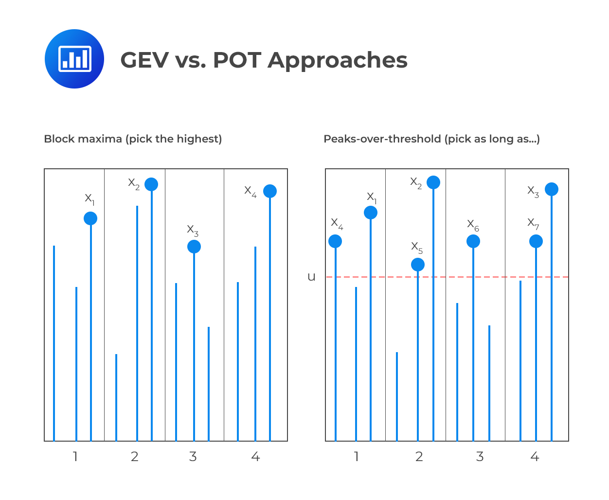
The figure below compares the generalized extreme value approach and the peaks-over-threshold approach. On the left, we can see that the GEV concerns itself with selected observations that are maxima of groups of three. On the right, we can see that the POT approach concerns itself with all observations that are greater than u. Notably, some of the observations ignored in the GEV (block maxima) approach make the cut in the POT approach.
 In practice, risk analysts prefer the POT approach to the GEV approach because the former is more efficient in the use of data. In other words, the GEV approach involves some loss of useful data relative to the POT approach, because some blocks might have more than one extreme in them. In addition, the POT approach is better adapted to the risk measurement of tail losses because it focuses on the distribution of exceedances over a threshold.
However, the POT approach comes with the problem of choosing a threshold, a situation that does not arise with the GEV approach.
At the end of the day, however, the choice between the two boils down to the problem at hand. A lot will depend on the amount of data available.
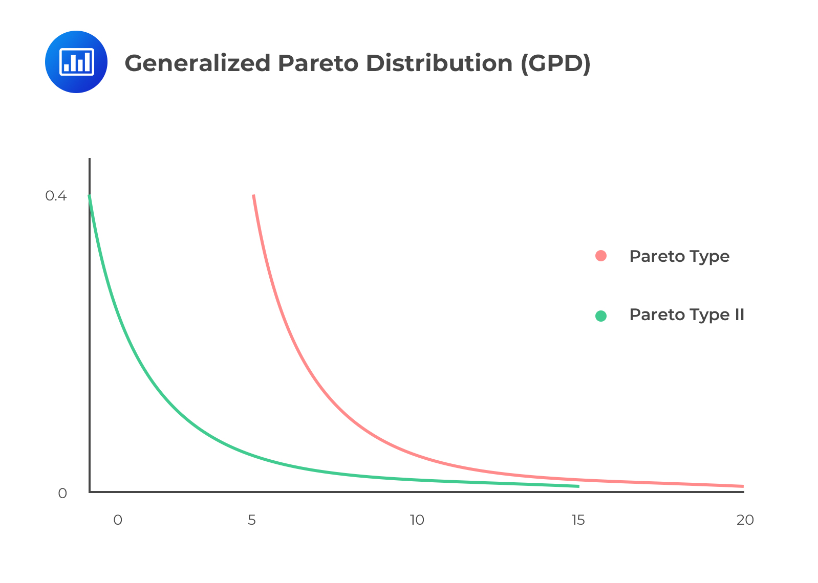
As u gets large, the Gnedenko–Pickands–Balkema–DeHaan (GPBdH) theorem states that the distribution \(\text{Fu(x)}\) converges to a generalized Pareto distribution, given by:
$$ \text G_{\xi,\beta} (\text x)=1-\left(1+\cfrac {\xi {\text x}}{\beta} \right)^{-\frac{1}{\xi}}\text { if } \xi \neq 0 $$
and,
$$ \text G_{\xi,\beta} (\text x)=1-\text{exp} \left(-\cfrac {\text x}{\beta} \right) \text { if } \xi = 0 $$
For these equations to hold, \({\text x} \ge 0\) for \(\xi \ge 0\) and \(0 \le {\text x}-\frac {\beta}{\xi}\) for \(\xi < 0\).
As seen above, the generalized Pareto distribution (GPD) has only two parameters:
 The GPD is considered the natural model for excess losses since all distributions of excess losses converge to the GPD. To apply the GPD, however, we need to choose a reasonable threshold u, which determines the number of observations, \(\text N_{\text u}\), in excess of the threshold value. But the process involves a trade-off. On the one hand, we have to come up with a threshold that is sufficiently high for the GPBdH theorem to apply reasonably closely. On the other, we have to be careful not to settle on a value that’s so high that it leaves us with an insufficient number of excess-threshold observations that lead to unreliable estimates.
Ultimately, the goal of the POT approach is to compute the value at risk. Once we have VaR estimates, we can proceed to derive the expected shortfall (conditional VaR). Remember that the expected shortfall is simply the average of all losses greater than the VaR.
Using POT parameters, we can compute the VaR as follows:
$$ \text{VaR}=\text u+ \cfrac {\beta}{\xi} \left\lceil \left[\cfrac {\text n}{\text N_{\text u}} \left( 1-\text{confidence level} \right) \right]^{-\xi}-1 \right\rceil $$
Where:
u = Threshold (in percentage terms).
N= Number of observations.
\(\text N_{\text u}\) = Number of observations that exceed the threshold.
The expected shortfall can then be defined as:
$$ \text{ES}=\cfrac {VaR}{1-\xi)}+\cfrac {\beta-\xi u}{1-\xi} $$
Assume the following observed parameter values:
Compute the VaR at 99% confidence and the corresponding expected shortfall.
$$ \begin{align*} \text{VaR} & =\text u+\cfrac {\beta}{\xi} \left\lceil \left[ \cfrac {\text n}{\text N_{\text u}} (1-\text{confidence level}) \right]^{-\xi}-1 \right\rceil \\ \text {VaR}_{0.99} & =1+\cfrac {0.6}{0.3} \left\lceil \left[ \cfrac {1}{0.05} (1-0.99) \right]^{-0.30}-1 \right\rceil=2.2413\% \\ \text{ES} & =\cfrac{\text{VaR}}{1-\xi}+\cfrac {\beta-\xi {\text u}}{1-\xi} \\ & =\cfrac {2.2413}{1-0.3}+\cfrac {0.6-0.3×1}{1-0.3}=3.6304\% \\ \end{align*} $$
In hydrology and meteorology, we may be interested in the joint flooding of two rivers, a scenario that puts the facilities (and people) living downstream at risk. Similarly, we could be interested in the simultaneous occurrence of high-speed wind and a wildfire, which can have disastrous effects on all forms of life. In finance, we can also be interested in the joint occurrence of two or more extreme events. For example, a terrorist attack on oil fields may lead to heavy losses for oil producers as well as a negative effect on financial markets. Multivariate extreme value theory seeks to establish the probabilities of extreme joint events.
Just as with univariate EVT, multivariate ETV concerns itself with the estimation of extreme events that lie far away from central, more common events. The only added feature is that we now apply EVT to more than one random variable at the same time. This leads us to the concept of tail dependence.
Tail dependence refers to the clustering of extreme events. In financial risk management, clustering of high-severity risks can have a devastating effect on the financial health of firms and this makes it an important part of risk analysis. It is generally agreed that tail dependence is independent of marginal distributions of the risks and is instead solely dependent on copulas. In other words, tail dependence cannot be sufficiently described by correlation alone.
Extreme-value copulas provide appropriate models for the dependence structure between extreme events. According to multivariate extreme value theory (MEVT), the limiting distribution of multivariate extreme values must be a member of the family of EV copulas. The task of modeling multivariate EV dependence, therefore, boils down to picking one of these EV copulas.
In theory, a single copula can have as many dimensions as the random variables of interest, but there’s a curse of dimensionality in the sense that as the number of random variables considered increases, the probability of a multivariate extreme event decreases. For example, let’s start with the simple case where there are only two independent variables and assume that univariate extreme events are those that occur only once for every 100 observations. In these circumstances, we should expect to see one extreme multivariate event (both variables taking extreme values) only once in 100<sup>2</sup>; that’s one time in 10,000 observations. If we work with three independent variables, we should expect to see an extreme multivariate event once in 100<sup>3</sup>; that’s once in 1,000,000 observations. This clearly shows that as the dimensionality rises, multivariate extreme events become rarer. That implies that we have a smaller pool of multivariate extreme events to work with, and more parameters to estimate. As such, analysts are forced to work with a small number of variables at a time.
Based on this information, it would be tempting to conclude that multivariate extremes are so sufficiently rare that we need not worry about them. Nothing could be farther from reality. There’s empirical evidence that (at least some) extreme events are not independent. For example, major earthquakes have in the past triggered other natural or financial disasters (e.g., tsunamis and market crashes). As we saw at the beginning of the topic, for example, the Kobe earthquake of 1995 had a serious impact on Asian financial markets, with the Nikkei registering a large drop. If you recall, Barings bank filed for bankruptcy after one of its traders, Nick Leeson, suffered huge losses in his bets against a fall in the Nikkei. In his assessment, there was a near-zero chance of the Nikkei losing more than 5% of its value. When the Kobe earthquake struck, the Nikkei lost more than 7%, resulting in severe losses for the bank.
Bottom line: Disasters are often related, and it is important for risk managers to have some awareness of extreme multivariate risks.
Question 1
Assuming that we are given the following parameters based on the empirical values from contracts on futures clearing companies: \(\beta=0.699\),\(\xi=0.149\),\(u= 3.3\),\({ { N }_{ u } }/{ n }=5.211\%\).Determine the VaR and expected shortfall (ES) at the 95.5% level of confidence, respectively.
1.674, 2.453
3.404, 4.243
1.453, 2.420
1.667, 2.554
The correct answer is B.
Recall that: $$ VaR=u+\frac { \beta }{ \xi } \left\{ { \left[ \frac { n }{ { N }_{ u } } \left( 1-\alpha \right) \right] }^{ -\xi }-1 \right\} $$ $$ ES=\frac { VaR }{ 1-\xi } +\frac { \beta -\xi u }{ 1-\xi } $$ Therefore: $$ VaR=3.3+\frac { 0.699 }{ 0.149 } \left\{ { \left[ \frac { 1 }{ 0.05211 } \left( 1-0.955 \right) \right] }^{ -0.149 }-1 \right\}= 3.4037 $$ $$ ES=\frac{ 3.4037 }{ 1-0.149 } +\frac{ 0.699-0.149\times 3.3 }{ 1-0.149}=4.2432 $$
Question 2
Samantha, a risk manager at Meridian Investments, is assessing the extreme risks in a highly complex portfolio containing multiple asset classes across various geographic locations. Samantha decides to employ the peaks-over-threshold (POT) approach to model extreme values beyond a specific threshold. She gathers substantial data over multiple decades and carefully selects a threshold that suits the analysis.
Samantha knows that applying the POT method requires a solid understanding of various statistical components, including the selection of the threshold, fitting the data, and extrapolation to more extreme values. She also recognizes that improper application could lead to misleading results.
Given this context, which of the following statements best describes the proper application of the POT approach in Samantha’s scenario?
A. The threshold must always be set at the highest observed value to capture the most extreme events.
B. The POT approach assumes that excesses over the threshold are distributed according to the normal distribution.
C. The threshold selection must balance between bias and estimation error by avoiding overly high or low thresholds.
D. The POT approach considers only values below the threshold, excluding all values that exceed it.
Solution
The correct answer is C.
The POT approach involves selecting a threshold, and the distribution of exceedances over this threshold is then modeled. The threshold selection must carefully balance between bias (from setting it too high) and estimation error (from setting it too low). Too high a threshold leads to few data points for analysis, increasing the error, while too low a threshold may lead to bias as non-extreme values are included.
A is incorrect because setting the threshold at the highest observed value would not leave any exceedances to model. The POT method requires a balance in threshold selection, and choosing the highest observed value would defy that principle.
B is incorrect because the POT approach typically assumes that excesses over the threshold are distributed according to the Generalized Pareto Distribution (GPD), not the normal distribution. This assumption is vital in modeling the tails of the distribution, where extreme values are often found.
D is incorrect because the POT approach focuses specifically on values that exceed the selected threshold. It does not consider only values below the threshold. The method aims to model what happens beyond a certain extreme point, and ignoring values that exceed the threshold would defeat this purpose.
Things to Remember
- The Peaks-over-Threshold (POT) approach is used to model extreme values beyond a specific threshold.
- Proper threshold selection is key. It should neither be too high nor too low.
- Too high a threshold results in fewer data points for analysis, which increases estimation error.
- Too low a threshold can introduce bias, as non-extreme values might be considered.
- Excesses over the threshold in the POT approach are typically modeled using the Generalized Pareto Distribution (GPD) rather than the normal distribution.
- The main focus of the POT method is on values that exceed the chosen threshold.
- Understanding statistical components, such as threshold selection, data fitting, and extrapolation, is crucial for the accurate application of the POT method.
Get Ahead on Your Study Prep This Cyber Monday! Save 35% on all CFA® and FRM® Unlimited Packages. Use code CYBERMONDAY at checkout. Offer ends Dec 1st.