Spread Risk and Default Intensity Models

After completing this reading, you should be able to:

• Compare the different ways of representing credit spreads.
• Compute one credit spread, given others when possible.
• Define and compute the Spread ‘01.
• Explain how default risk for a single company can be modeled as a Bernoulli trial.
• Explain the relationship between exponential and Poisson distributions.
• Define the hazard rate and use it to define probability functions for default time and conditional default probabilities.
• Calculate the unconditional default probability and the conditional default probability given the hazard rate.
• Distinguish between cumulative and marginal default probabilities.
• Calculate risk-neutral default rates from spreads.
• Describe the advantages of using the CDS market to estimate hazard rates.
• Explain how a CDS spread can be used to derive a hazard rate curve.
• Explain how the default distribution is affected by the sloping of the spread curve.
• Define spread risk and its measurement using mark-to-market and spread volatility.

The Different Ways of Representing Credit Spreads

Informally, a credit spread is the difference in yield between two bonds of similar maturity but different credit quality. For example, the credit spread between a 10-year Treasury bond trading at a yield of 5% and a 10-year corporate bond trading at 8% is 3%. In this case, the corporate bond is said to be trading at a 300-basis-point spread over the T-bond. Represented graphically over time, it could look like the following illustration:

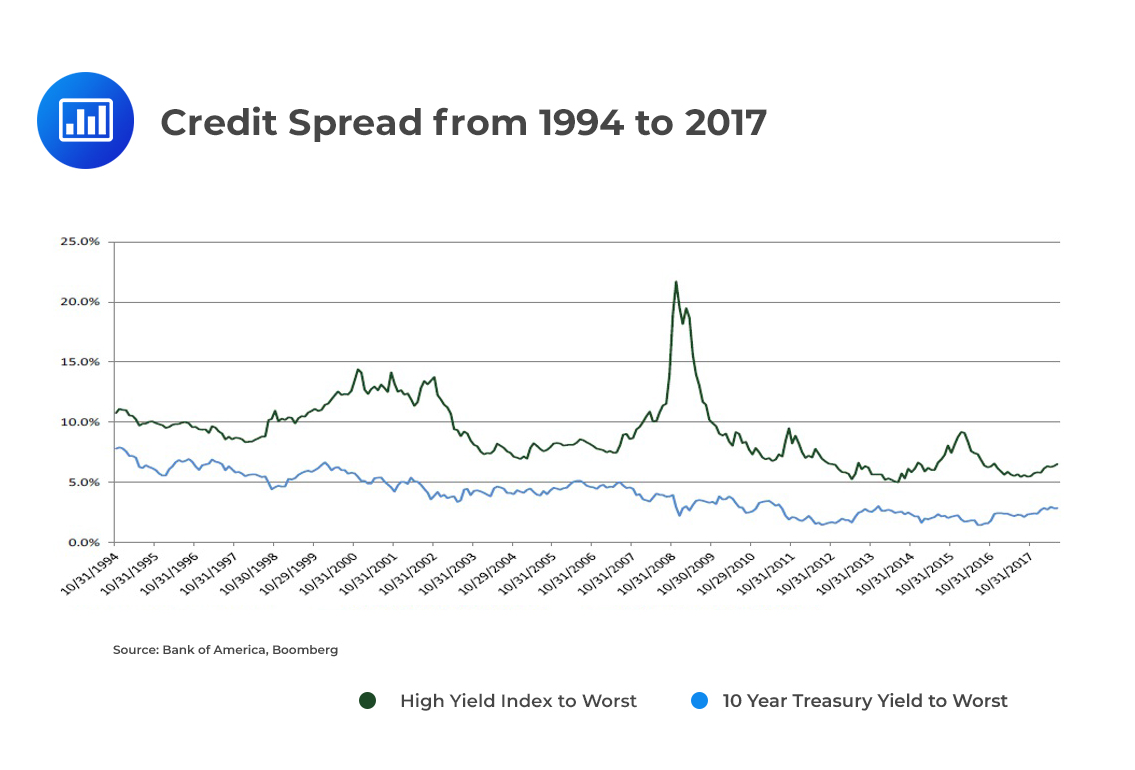We can represent the risk-free rate in several ways – as spot rates, forward rates, or even discount factors. Likewise, we can represent credit spreads in a number of different ways. Each of these credit spreads attempts to break down bond interest into two:

1. Compensation for credit and liquidity risk.
2. Compensation for the time value of money (TVM).

Let’s now look at the various spread measures:

Yield Spread

Yield spread is the difference between the YTM of a credit-risky bond and that of a benchmark government bond with the same or approximately the same maturity.

$$ \text{Yield spread} = \text{YTM[risky bond, maturity T]} – \text{YTM[riskless government bond, maturity T]} $$

Yield spreads are commonly used in price quotes but are featured, to a lesser extent, in fixed-income analysis.

Interpolated Spread

In most cases, it is not possible to find a zero-risk security of the same maturity as a credit-risky bond. For this reason, analysts tend to estimate the spread by extrapolating the yield of risk-free securities whose maturities flank that of the risky debt.

Interpolated spread (i-spread), therefore, can be defined as the difference between the yield of a credit-risky bond and the linearly interpolated yield for the same maturity on an appropriate reference yield curve.

As with the yield spread, the i-spread is commonly used in price quotes.

Z-spread

The Z-spread is the basis-point spread that would need to be added to the LIBOR spot yield curve such that all the discounted cash flows of a bond are equal to its present value (current market price of the bond). In some instances, LIBOR is not used. Worth noting is the fact that the z-spread is measured relative to a government bond curve. For this reason, it is imperative to specify the reference risk-free curve being used.
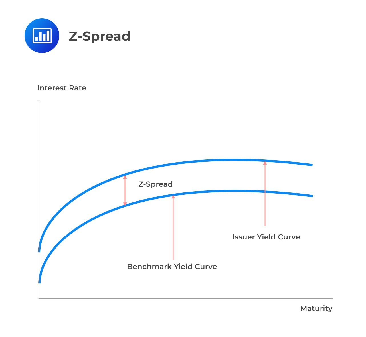The z-spread is the z that satisfies the following equation:

$$ {\text {p} }_{ \tau ,\text h }\left(\text C \right) =\text {ch}\sum _{\text i=1 }^{ \cfrac { \tau }{\text h } }{ {\text e }^{ -\left( {\text r }_{ \text {ih} }+\text z \right) \text {ih} } } +{ \text e }^{ -\left( {\text r }_{ \tau }+{\text z} \right) \tau } $$

Where:

\({\text {p} }_{ \tau ,\text h }\left( \text C \right)\) = Price of a credit-risky bond.

\({\tau}\) = Time to maturity in years.

c = Coupon.

h = Payment frequency.

Asset-swap Spread

This is the spread or quoted margin on the floating leg of an asset swap on a bond.

Credit Default Swap Spread

This is the market premium, expressed in basis points, of a CDS on similar bonds of the same issuer.

Option-adjusted Spread

This is a version of the z-spread that takes options embedded in a bond into account. It is only identical to the z-spread if no options are contained in the bond.

Discount Margin

Discount margin (also called quoted margin) is a concept applied to floating rate notes. It refers to the fixed spread over the current (one-or three-month) LIBOR rate that prices the bond precisely.

Example 1: Computing the Yield Spread

Assume we have the following two bonds: one issued by ABC Company and the other by the U.S Treasury

$$ \begin{array}{c|c|c|c|c|c} \textbf{Bond} & {\textbf{Coupon rate} \\ \textbf{(semiannual)}} & {\textbf{Time to} \\ \textbf{maturity}} & \textbf{Price} & \textbf{YTM} & {\textbf{Yield} \\ \textbf{curve}}\\ \hline {\text{ABC}} & {10\%} & {10} & {95} & {10.49\%} \\ \hline {\text{U.S. Treasury}} & {6\%} & {10} & {97} & {6.69\%} & {6\%\text{Flat}}\\ \end{array} $$

Compute the yield spread.

Solution

$$ \text{Yield spread} = 10.49\% – 6.69\% = 3.8\% = 380 \text{ basis points} $$

Example 2: Computing the i-spread

$$ \begin{array}{c|c|c|c|c|c} \textbf{Bond} & {\textbf{Coupon rate} \\ \textbf{(semiannual)}} & {\textbf{Time to} \\ \textbf{maturity}} & \textbf{Price} & \textbf{YTM} \\ \hline {\text{ABC}} & {10\%} & {9} & {95} & {10.49\%} \\ \hline {\text{U.S. Treasury 1}} & {6\%} & {10} & {97} & {6.69\%} \\ \hline {\text{U.S. Treasury 2}} & {5\%} & {8} & {97} & {5.47\%} \\ \end{array} $$

Compute the i-spread.

Solution

Because the maturity of the ABC bond (9 years) does not exactly match exactly the maturity of the quoted Treasury bonds (8 and 10 years), the i-spread will be calculated as follows:

i-spread = YTM of ABC – Linearly interpolated YTM of Benchmark Treasuries

$$ \text{i-spread} = 10.49\% −\frac{(6.69\%+5.47\%)}{2}=4.41\%$$

Spread01

In the context of interest rates, remember that DV01 is the price increase (“mark-to-market gain”) implied by a one basis point decline in interest rate. Spread01 is an analogous concept. It is a measure of the change in the value of a credit-risky bond for a one basis point change in spread. Spread01 is also called DVS1.

For a credit-risky bond, spread01 is measured as the change in the market value corresponding to a one basis point change in the z-spread. The steps involved are as follows:

1. Increase the z-spread by 0.5 basis points and determine the price of the bond.
2. Decrease the z-spread by 0.5 basis points and, again, re-price the bond.
3. Compute the difference.

Example: Computing the Spread01

Assume that the current price of a bond is $92.45, and the z-spread currently stands at 202 basis points. The z-spread is increased and decreased by a 0.5 basis point margin, and the price changes to $92.35 and $92.56, respectively. Determine the spread01 per $100 par value.

Solution

Spread01 = $92.56 – $92.35 = $0.21 per basis point

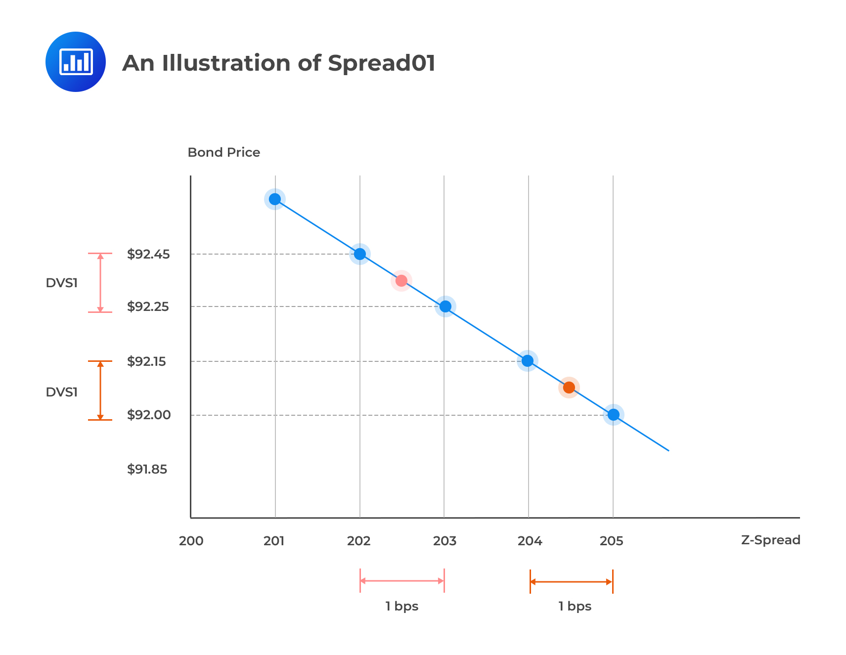Spread01 exhibits convexity; any increase or decrease in the spread has a smaller impact on a bond’s value when spreads are higher and the discount factor is lower.

Modeling Default Risk as a Bernoulli Trial

The default risk of a single obligor (company) can be modeled as a Bernoulli trial. Remember that a Bernoulli trial is an experiment where the outcome can take on only two values: success or failure (i.e., a binomial distribution). Over some fixed horizon \({ \tau }\) = \( { \text T }_{ 2 }- {\text T }_{ 1 }\), there are two possible outcomes:

• Default occurs with a probability \(\pi\).
• The firm remains solvent with probability \(1-\pi\).

We could assign values 1 and 0 to default and solvency over the horizon \({ \tau }\) =\( {\text T }_{ 2 }- {\text T }_{ 1 }\). By so doing, we define a random variable that follows the Bernoulli distribution. Note that the time horizon is always specified. We are interested in the probability of default over a specified period of time, say, 1 year. The mean and variance of a Bernoulli distribution are equal to \(\pi\) and \(\pi(1-\pi)\), respectively.

A key property under the Bernoulli distribution is that each trial is considered conditionally independent; that the probability of default in period t is independent of default in period t-1 and all other previous periods.

The Relationship between Exponential and Poisson Distributions

Computing the probability of default over a discrete number of periods is relatively straightforward. For example, if we set the probability of default equal to 5% working with one-year periods, the probability of survival over the next decade is:

$$ \text {P(survival)} = { \left( 1-\pi \right) }^{ 10 }= { ( 1-5\%) }^{ 10 } = 59.9\% $$

The Bernoulli distribution works really well when modeling default over discrete time periods but is a rather inconvenient choice when we wish to model default over time. For example, we may want to establish the total number of defaults in the first 10 years of a bank’s existence.

One viable alternative is to use the Poisson model where the random time at which default occurs is modeled as the first arrival time – the time at which the event occurs.

Under the Poisson model, the number of events in any time interval is Poisson-distributed.

$$ {\text P}\left( \text X =\text x \right) =\left( \cfrac { { \lambda }^{\text x }{\text e }^{ -\lambda } }{ \text x ! } \right) \\ $$

Where:

x = Number of successes (defaults) per unit.

\({ \lambda }\) = Average/expected number of successes per unit.

The time to the next event (arrival) is described by the exponential distribution.

Hazard Rate

The hazard rate (also called default intensity) is the probability of default for a certain time period conditional on no earlier default. It is the parameter driving default. It is usually represented by the parameter \(\lambda\). The probability of default over the next small time interval, dt, is \({ \lambda }\text {dt}\).

$$ \text{PD} \left( \text t,\text t+{\text {dt}} \right)={ \lambda } \text{dt} $$

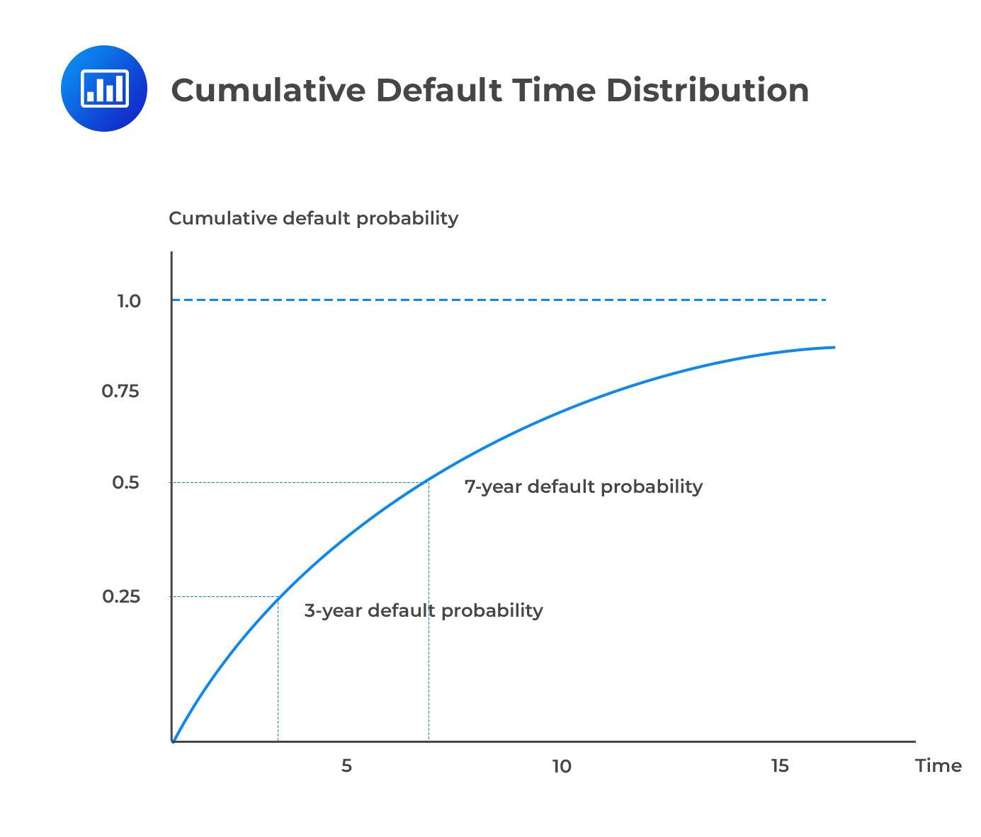
Using \({\text t }^{ * }\) to represent the time of default, the cumulative default time distribution F(t) gives the probability of default over (0,t).

$$ \text P\left[ { \text t }^{ * }< {\text t} \right] \equiv {\text F}(\text t)=1-{ \text e }^{ -\lambda {\text t} } $$

The survival distribution is as follows:

$$ {\text P}\left[ { \text t }^{ * }\ge {\text t} \right] =1-{\text P}\left[ {\text t }^{ * }<\quad {\text t} \right] =1-{\text F}\left( \text t \right) { =\text e }^{ -\lambda {\text t} } $$

Note that the default time distribution and the survival distribution add up to 1 at each point in time.

As t grows very large, the survival probability converges at 0 while the default probability converges at 1. The intuition is that the probability of default increases as we peer deeper into the future. Even the best-rated bond, say AAA, will eventually default.

$$ \textbf{Default Time Density Function} $$

The default time density function is the derivative of the default time distribution, w.r.t t. Sometimes, it is called the marginal default probability.

$$ \cfrac { \partial }{ \partial {\text t} } {\text P}\left[ {\text t }^{ * }< {\text t} \right] ={ \text F }^{ \prime \left(\text t \right) }=\lambda { \text e }^{ -\lambda {\text t} }$$

The default time density function is always positive because default risk tends to “accumulate” over time. However, the rate of increase depends on \({\lambda}\). With a big value, default risk will increase at a quick pace.

The survival probability, again, decreases over time.

$$ \cfrac { \partial }{ \partial {\text t} } {\text P}\left[ { \text t }^{ * }\ge {\text t} \right] ={ -\text F }^{ \prime \left( \text t \right) } =-\lambda { \text e }^{ -\lambda {\text t} } $$

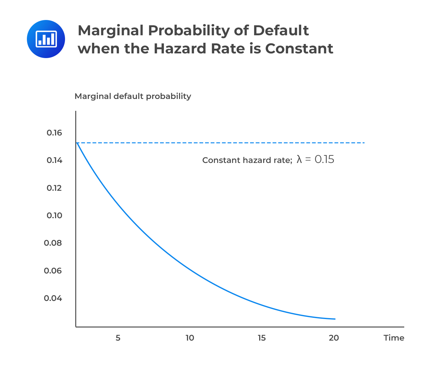
If we hold the hazard rate at a constant value \({\lambda}\), we will find that the marginal default probability is positive but declining. The implication is that although the probability of default increases the further out we peer into the future, the rate at which this probability accumulates declines.

$$ \textbf{Conditional Default Probability} $$

The conditional default probability gives the probability of default over some horizon \((\text t,\text t+\tau)\) given that there has been no default prior to time t.

$$ \text P\left( { \text t }^{ * } < {\text t}+\tau |{ \text t }^{ * } > {\text t} \right) =\cfrac { \text p\left[ {\text t }^{ * } > \text t\cap { \text t }^{ * } < {\text t}+\tau \right] }{ \text p \left[ { \text t }^{ * } > {\text t} \right] } \ $$

For example, the conditional one-year probability of default, assuming survival during the first year, is equal to the difference between the unconditional two-year PD and the unconditional one-year PD divided by the one-year survival probability.

$$ \text{Conditional one year PD} \\ =\cfrac { \text{Unconditional two year PD-unconditional one year PD} }{ \text{one year survival PD} } $$

Example: Computing the Conditional PD

Compute the one-, two-, and three-year cumulative default probabilities and conditional default probabilities, assuming that the hazard rate is 0.10

Solution

$$ \textbf{Conditional Default Probability} $$

\(\quad \quad \quad \textbf{Hazard Rate,} \bf{\lambda = 0.1} \)

$$ \begin{array}{c|c|c|c|c} \bf{\text t} & {\textbf{Cumulative PD} \\ {\left[ 1-{ \text{e} }^{ -\lambda \text{t} } \right] } } & {\textbf{Survival Prob.} \\ {\left[{ \text{e} }^{ -\lambda \text{t} } \right] } } & \textbf{PD(t,t+1))} & {\textbf{Conditional PD} \\ \textbf{given survival until} \\ \textbf{time t} } \\ \hline 1 & {1-{ \text{e} }^{ -0.1\times 1 } \\ {=9.52\%} } & {{ \text{e} }^{ -0.1\times 1 } \\ {=90.48\%} } & {9.52\%} & {-} \\ \hline 2 & {1-{ \text{e} }^{ -0.1\times 2 } \\ {=18.13\%} } & {{ \text{e} }^{ -0.1\times 2} \\ {=81.87\%} } & { \left( 18.13\%-9.52\% \right) \\ {=8.61\%} } & { {\frac {8.61\%}{90.48\%} } \\ {=9.52\%} } \\ \hline 3 & {1-{ \text{e} }^{ -0.1\times 3 } \\ {=25.92\%} } & {{ \text{e} }^{ -0.1\times 3} \\ {=74.08\%} } & { \left( 25.92\%-18.13\% \right) \\ {=7.79\%} } & { {\frac {7.79\%}{81.87\%}} \\ {=9.52\%} } \end{array} $$

Notice that the two conditional probabilities are equal.

Risk-neutral Default Rates

Default probabilities can also be extracted from market prices. The resulting probabilities are risk-neutral. This implies that the probabilities include compensation for both the loss given default and bearing the risk of default and uncertainties that come along with it.

The spread over the risk-free rate on a bond that is defaultable with maturity T is denoted by \(\text z_{\text t}\), and the constant risk-neutral hazard rate at time T is \(\lambda_{\text T}^{*}\).

If recovery is zero,

$$ { \lambda }_{ \text T }^{ * }={ \text z }_{ \text t } $$

The equation above implies that the hazard rate is equal to the spread.

For small values of x, we can use the approximation \(\text e^{\text x}=1+ \text x\) so that:

$$ { \text z }_{\text t }=1-{\text e }^{ -{ \lambda }_{\text T }^{ * } } $$

After a bit of algebraic manipulation, it can be shown that the average default intensity over the life of the bond is approximately,

$$ \cfrac { \text S }{ 1-{\text R} } $$

where s is the spread of the bond’s yield over the risk-free rate and R is the recovery rate.

Example: With a five-year bond that has a spread of 200 bps and a recovery rate of 40%, for example, the average default intensity (hazard rate) = 0.02/0.6 = 0.0333.

Estimating Hazard Rates from CDS Markets

In practice, corporations rarely issue zero-coupon bonds. In such circumstances, it becomes difficult to estimate hazard rates using bond prices. Most zero-coupon corporate issues are in form of commercial paper that matures in less than one year, and even these are issued by “blue chip” companies with impeccable financial reputations. For this reason, hazard rates are often estimated from the CDS prices.

Advantages

Standardization

The bond market is so diverse that cash flows and seniority in the event of winding up are significantly different. Therefore, it is difficult to come up with a default analysis model that takes all these differences into account. The CDS market does not have most of these problems. For instance, maturities are standardized (1, 3, 5, 7, and 10 years) with the five-year point generally the most liquid.

Coverage

CDSs can be issued on a wide range of reference entities. One of the largest CDS market purveyors, Markit Partners, provides curves on more than 3,800 CDS entities and millions of daily quotes covering 10,000+ CDS curves.

Liquidity

CDSs are more liquid than bonds. What’s more, the liquidity of CDS with different maturities is usually less than that of bonds of a given issuer.

Deriving a Hazard Rate Curve from CDS Spread

Before looking at how we can go about deriving a hazard rate curve from CDS spread, let’s remind ourselves of a few things about credit default swaps.

Generally, no principal or other cash flows change hands at the initiation of the contract.

However, when CDS trade points upfront, a percent of the principal is paid by the protection buyer. This impacts the counterparty credit risk of the contract rather than its pricing. In addition, some collateral has to be provided at the onset.

Each contract has a set of agreed future cash flows.

Quarterly spread payments (called the free leg) have to be made by the protection buyer until the maturity date of the contract, unless and until the reference entity undergoes an event of default.

The protection seller makes a payment, called the contingent leg, only if there is a default. This payment leg is equal to the loss given default.

The pricing of the CDS is set so that the expected net present value of the CDS contract is zero.

At the onset, the expected present value of the free leg is equal to that of the contingent leg.

The Derivation Process

Assume that we wish to find the default curve for a company. Let’s further assume that we have only a single CDS spread, for a term of five years. As such, we will have a single hazard estimate. The protection buyer will pay the spread in quarterly installments. These will be dates t = 0.25, 0.5,…1.5, 5. The installments will be a function of the unknown hazard rate λ, which is linked to the probability of survival up to time t, \({ \pi }_{ \text t }\), as follows:

$$ { \pi }_{\text t }=1-{\text e }^{ -\lambda {\text t} } $$

We will need to work with the CDS valuation equation which equates the PV of the free leg to the PV of the contingent leg.

The PV of the free leg is given by:

$$ \cfrac { { \text S }_{ \tau } }{ 4\times { 10 }^{ 4 } } \sum _{ \text u=1 }^{ { 4 }{ \tau } }{ { {\text p }_{ 0.25{\text u} } } } \left[ { \text e }^{ -\lambda \left( \cfrac { \text u }{ 4 } \right) }+0.5\left( { \text e }^{ -\lambda \cfrac { \left( \text u-1 \right) }{ 4 } }-{ \text e }^{ -\lambda \left( \cfrac { \text u }{ 4 } \right) } \right) \right] $$

While the PV of the contingent leg is given by:

$$ \left( 1-\text R \right) \sum _{\text u=1 }^{ { 4 }{ \tau } }{ { { \text p }_{ 0.25{\text u} } } } \left( {\text e }^{ -\lambda \cfrac { \left( \text u-1 \right) }{ 4 } }-{\text e }^{ -\lambda \left( \cfrac { \text u }{ 4 } \right) } \right) $$

where:

• \({ \text p }_{ \text t }\) is the price of a risk-free zer0-coupon bond maturing at time t.
• R is the recovery rate = 1 – LGD.
• \({ \pi }_{ \text t }\) is the probability of survival up to time t.
• \(\tau\) = Term of the CDS (5 in this example).
• \({ \text S }_{ \tau }\) = Spread of the CDS.
• \({\lambda}\) = Hazard rate (our unknown).

Provided all the variables are known, we can substitute them in the equation and get the value of λ

Example: Single Hazard Rate

$$ \begin{array}{c|c} \textbf{Reference entity} & \textbf{Merrill Lynch} \\ \hline \text{Initiation Date} & \text{October 1 2008} \\ \hline {\text{Single five-year CDS spread}, \text s_\tau} & \text{445 bps} \\ \hline \text{Hazard Rate} & \text{Constant} \\ \hline \text{Recovery Rate, R} & {40\%} \\ \hline \text{Swap curve} & \text{Flat} \\ \hline \text{Continuously compounded spot rate} & {4.5\%} \\ \hline {\text{Term of the CDS}, \tau} & \text{5 years} \\ \end{array} $$

We can work out a value for \(\lambda\) as follows:

$$ \cfrac { 445 }{ 4\times { 10 }^{ 4 } } \sum _{\text u=1 }^{ { 4 }_{ \tau } }{ {\text e }^{ 0.045\left( \frac { \text u }{ 4 } \right) } } \left[ { \text e }^{ -\lambda \left( \frac { \text u }{ 4 } \right) }+0.5\left( { \text e }^{ -\lambda \frac { \left(\text u-1 \right) }{ 4 } }-{ \text e }^{ -\lambda \left( \frac { \text u }{ 4 } \right) } \right) \right] $$

$$ =\left( 1-0.4 \right) \sum _{ \text u=1 }^{ { 4 }{ \tau } }{ {\text e }^{ 0.045\left( \frac { \text u }{ 4 } \right) } } \left( {\text e }^{ -\lambda \frac { \left( \text u-1 \right) }{ 4 } }-{\text e }^{ -\lambda \left( \frac {\text u }{ 4 } \right) } \right) $$

Solving this gives \(\lambda\)=0.0741688

Example: Hazard Rate Curve

The hazard rate curve can be obtained via a bootstrapping process. The table below gives the closing CDS spreads for Merrill Lynch as of October 1, 2008.

As we did earlier, we assume a recovery rate of 40% flat swap curve, and a discount function \({ \text e }^{ 0045{\text t} }\).

$$ \begin{array}{c|c|c|c} \textbf{i} & \bf {\tau_{\text i} (\text{years})} & \bf {{\text S }_{ { \tau }_{ \text i } }( \text {bps/year})} & \bf {\lambda_{\text i}} \\ \hline {1} & {1} & {576} & {0.09600} \\ \hline {2} & {3} & {490} & {0.07303} \\ \hline {3} & {5} & {445} & {0.05915} \\ \hline {4} & {7} & {395} & {0.03571} \\ \hline {5} & {10} & {355} & {0.03416} \\ \end{array} $$

The forward hazard rates are extracted at each step i, using quarterly default probabilities over the given time interval by progressively “filling in” the integral equation as the bootstrapping process moves out the curve.

How Default Distribution is Affected by the Sloping of the Spread Curve

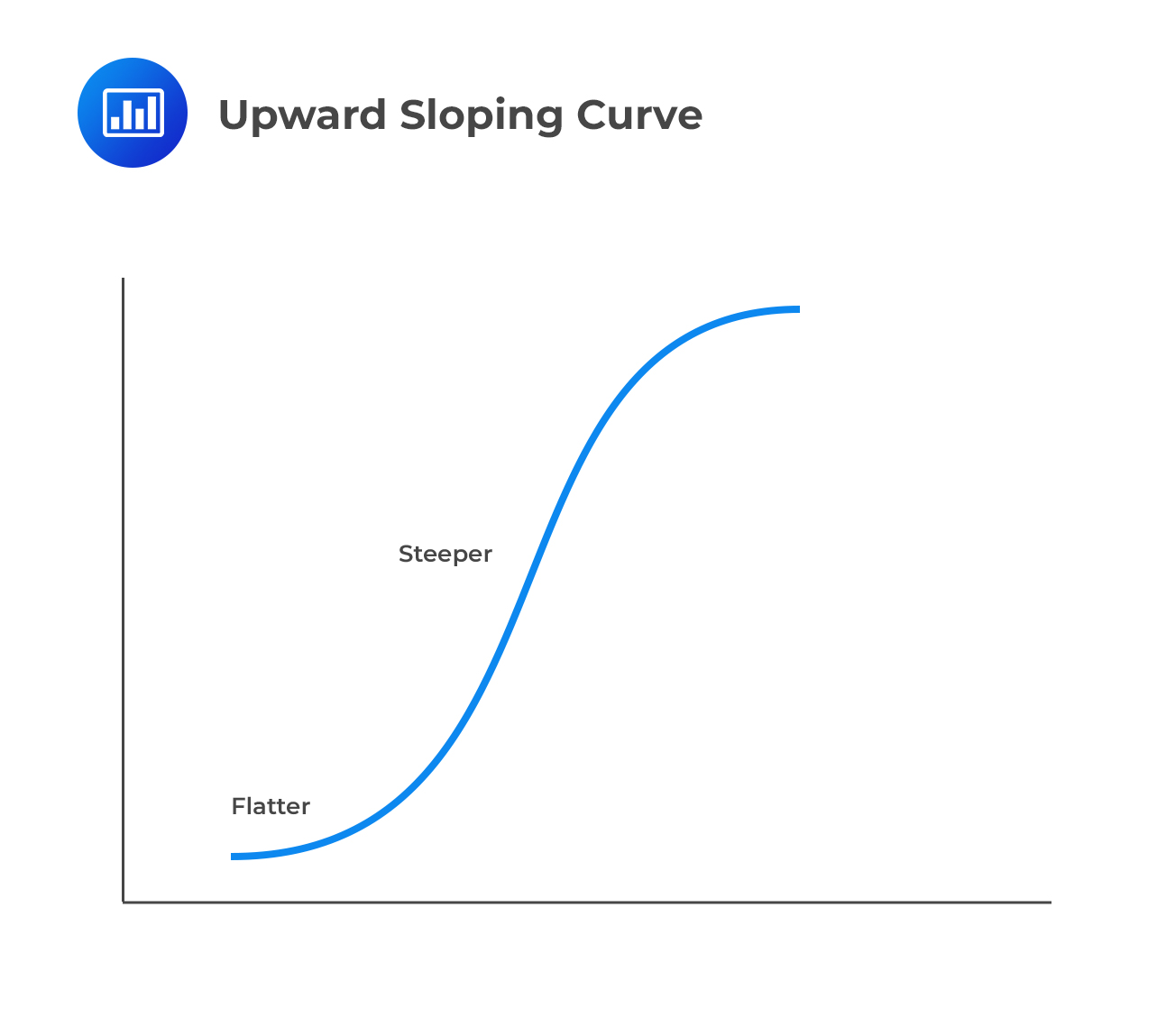
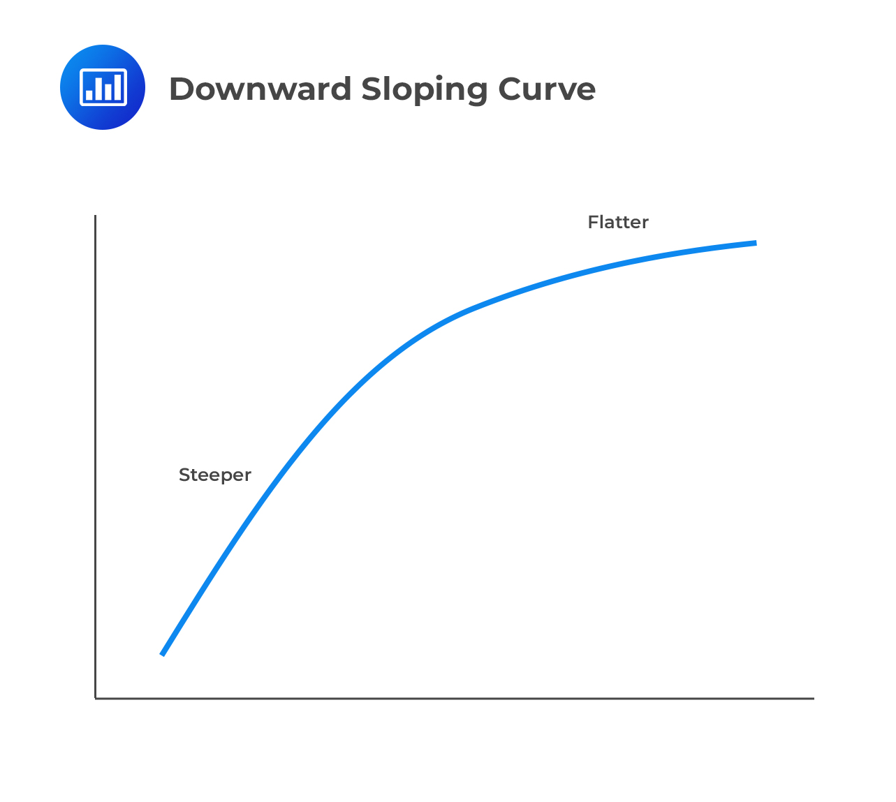
Spread curves, and thus hazard curves, may be upward or downward-sloping.

An upward-sloping curve is synonymous with a default distribution with the following characteristics:

• A relatively flat slope for shorter horizons.
• A steeper slope for more distant horizons.

What’s the intuition? the credit has a better risk-neutral chance of surviving the next few years thanks to a relatively low starting point for the hazard rate and therefore the unconditional default probability. However, the conditional probability of default (marginal probability) in future years falls less quickly (and sometimes even rises).

A downward-sloping curve is synonymous with a default distribution with the following characteristics:

• A relatively steep slope for shorter horizons.
• A flattening slope for more distant horizons.

What’s the intuition? if the firm survives the early, “dangerous” years, it has a good chance of surviving for a long time

The Typical Appearance of Spread Curves

Spread curves are typically gently upward-sloping. If the market has faith in a firm’s financial strength and believes that the default probability is low and stable, with a very small chance of significant change in the near future, the firm’s spread curve would be flat if it reflected default expectations only.

In reality, however, spreads also reflect some compensation for risk. For longer horizons, the likelihood of an unforeseen and unforeseeable change in a firm’s situation increases, triggering an increase in its default probability. A part of the increased spread for longer horizons is actually a risk premium that compensates for this possibility.

Downward-sloping spread curves are quite unusual and signify that the market views a credit as distressed. Downward-sloping curves were prevalent during the subprime mortgage crisis.

Spread Risk and its Measurement

Spread risk is the risk of loss from changes in the pricing of credit-risky securities. As noted previously, parties to a CDS implicitly agree on a fair swap spread such that that the expected payments to both are equal. If the swap spread changes at any point in the future, one of the parties suffers.

If the spread narrows (occasioned by improving the financial fortunes of the reference entity), it is the protection buyer who suffers because, at initiation, they locked in a premium that is now “above-market” and would not be payable based on current conditions.

If the spread widens (occasioned by the worsening financial fortunes of the reference entity), it is the protection seller who loses because, at initiation, they locked in a premium that is now “below-market” and would not be payable based on current conditions.

When measuring spread risk, there are two alternatives:

Marking-to-market

The marking-to-market effect is computed by shocking the entire CDS curve up and down by 0.5 basis points.

Note that this process bears similarities with the measurement of spread01, only that in this case, we execute a parallel shift up and down of the entire CDS curve by 0.5 bps, not just the z-spread (a single number).

We can also draw parallels between this process and the computation of the DV01 of a risk-free bond where the entire spot curve is shifted up or down by 0.5 bps.

Computing Spread Volatility

Spread volatility is the standard deviation—historical or expected—of changes in a spread, generally measured in basis points per day.

Practice Question

The probability of survival of a small financial institution is equal to 98% over one year. The probability of survival over the next three years is closest to which of the following?

A. 94%.

B. 95%.

C. 96%.

D. 98%.

The correct answer is A.

$$ \text {P(survival)} = { \left( 1-\pi \right) }^{ 3 }= { ( 1-2\%) }^{ 3 } = 94.12\% $$