After completing this reading, you should be able to:

• Define and calculate default correlation for credit portfolios.
• Identify drawbacks in using the correlation-based credit portfolio framework.
• Assess the impact of correlation on a credit portfolio and its Credit VaR.
• Describe the use of a single-factor model to measure portfolio credit risk, including the impact of correlation.
• Define and calculate Credit VaR.
• Describe how Credit VaR can be calculated using a simulation of joint defaults.
• Assess the effect of granularity on Credit VaR.

Default Correlation

When modeling a credit-risky position, there are a number of elements that we take into consideration. These include:

• The probability of default.
• The LGD and recovery rate.
• Rating migration probabilities.
• Spread risk.
• Possible eventual proceedings for a company in distress, such as the restructuring of debt.

A portfolio of credit instruments is exposed to a myriad of risks, just like any other portfolio. Although the probability of default of some two firms may be uncorrelated, default events do show some correlation. Default correlation measures the probability of multiple defaults for a credit portfolio issued by multiple obligors.

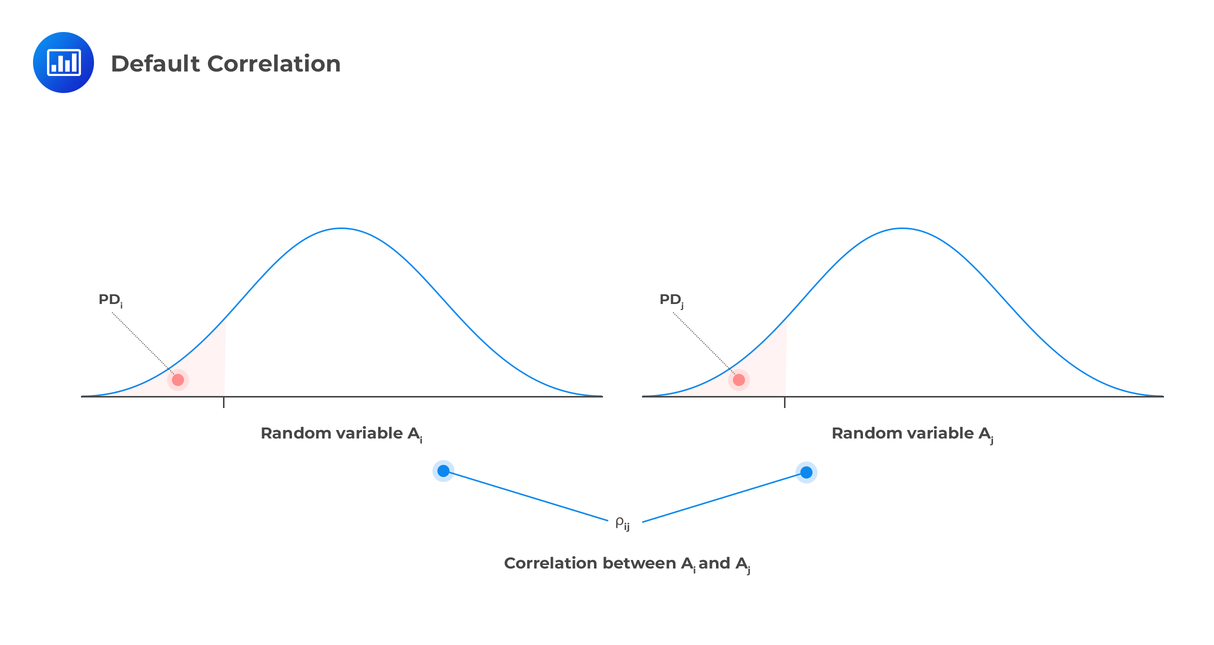To understand the concept of default correlation, let’s assume the following:

• We have positions in two firms.
• The probability of default (restructuring) is \({ \pi }_{ 1 }\) and \({ \pi }_{ 2 }\).
• The time horizon is \(τ\).
• The joint probability of default is \({ \pi }_{ 12 }\).

When modeling the credit risk of our two-firm position, we can interpret the portfolio as the distribution of the product of two Bernoulli-distributed random variables, \({ \text x }_{ i }\), with four possible outcomes. The table below illustrates this.

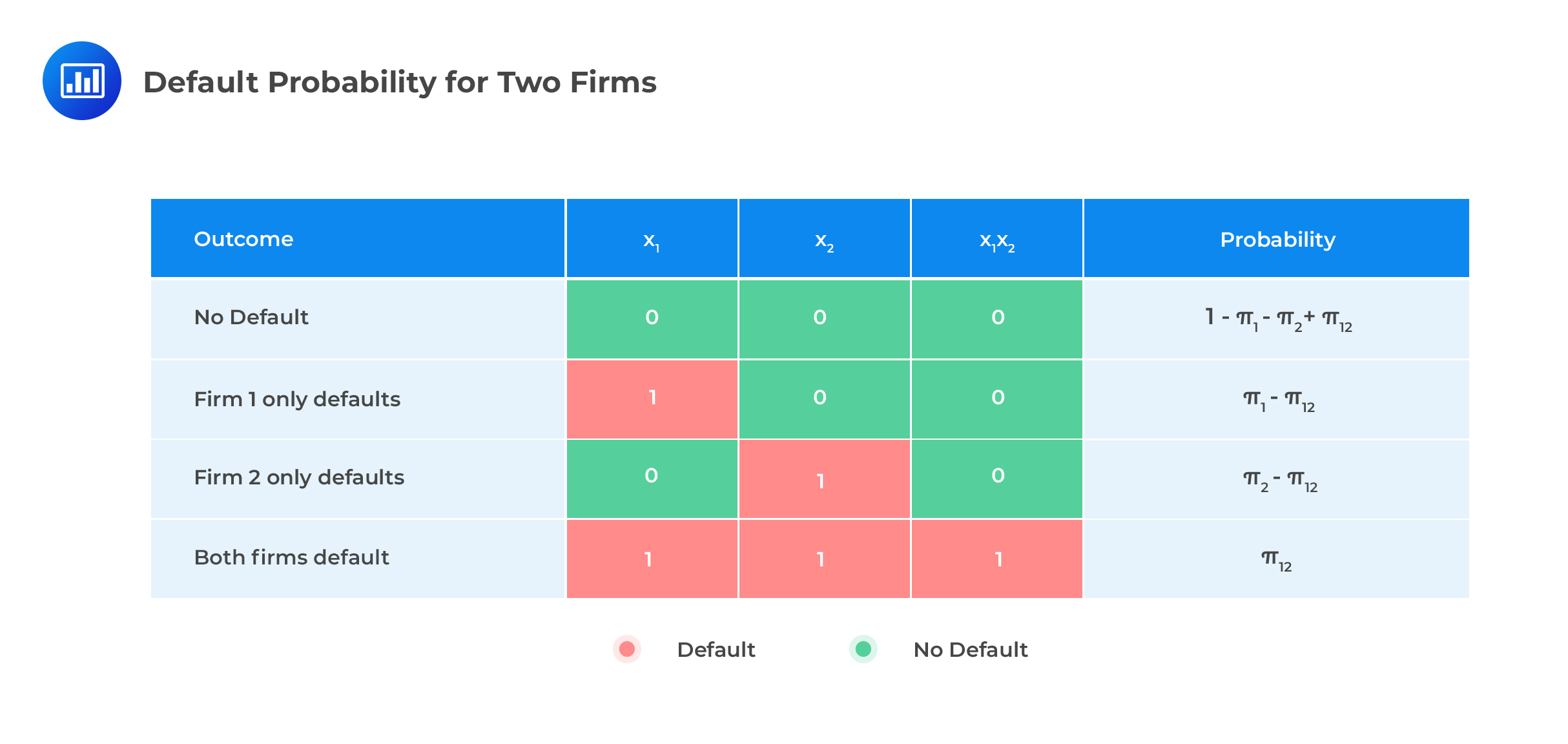We note a few points.

• All probabilities must add up to 1.
• The probability that at least one firm defaults can be determined in two ways. First, we can simply subtract the probability of the first outcome from 1. Alternatively, we can sum up the probabilities of the last three outcomes.

$$ \text{P} \left[ \text{Default by firm 1 or 2 or both} \right] ={ \pi }_{ 1 }+{ \pi }_{ 2 }-{ \pi }_{ 12} $$

To derive default correlation, let us consider the moments of Bernoulli-distributed default events:

The means of the two Bernoulli distributed default events are:

$$ \text{E} \left[ \text X_{ \text{i} } \right] ={ \pi }_{ \text{i} } , \text{ where i}=1, 2 $$

The expected value of the product (joint default) 0 is:

$$ \text{E} \left[ \text X_{ 1 } {\text X}_{ 2 } \right] ={ \pi }_{ 12 } $$

The variances are:

$$ \text{E} { \left[ \text X_{ \text{i} } \right] }^{ 2 }- \left(\text{E} { \left[ \text X_{ \text{i} } \right] } \right)^{ 2 }={ \pi }_{ \text{i} }\left( 1-{ \pi }_{ \text{i} } \right) , \text{ where i}=1, 2 $$

The covariance is:

$$ \text{E} \left[ {\text X}_{ 1 } {\text X}_{ 2 } \right] -\text{E} \left[ {\text X}_{ 1 } \right] { \text{E} \left[ {\text X}_{ 2 } \right] =\pi }_{ 12 }-{ \pi }_{ 1 }{ \pi }_{ 2 }$$

Finally, the default correlation is:

$$ \rho_{12}=\cfrac { { \pi }_{ 12 }-{ \pi }_{ 1 }{ \pi }_{ 2 } }{ \sqrt { { \pi }_{ 1 }\left( 1-{ \pi }_{ 1 } \right) } \sqrt { { \pi }_{ 2 }\left( 1-{ \pi }_{ 2 } \right) } } $$

If we treat the default correlation as a primitive parameter rather than the joint default probability, we could find the joint default probability:

$$ { \pi }_{ 12 }={ \rho }_{ 12 }\sqrt { { \pi }_{ 1 }\left( 1-{ \pi }_{ 1 } \right) } \sqrt { { \pi }_{ 2 }\left( 1-{ \pi }_{ 2 } \right) } +{ \pi }_{ 1 }{ \pi }_{ 2 } $$

If the two default events are independent, then the joint default probability is \( { \pi }_{ 12 }={ \pi }_{ 1 }{ \pi }_{ 2 }\), and the default correlation \({ \rho }_{ 12 }\)=0. As long as the default correlation is a value not equal to zero, there is a linear relationship between the probability of joint default and the default correlation.

Example: Calculating Default Correlation

An investment firm holds a position in two credits. The first credit is rated AAA with a probability of default of 0.001 over the next time horizon t. The second credit is rated BBB with a probability of default of 0.004 over a similar horizon. The joint probability of default over time horizon t is 0.00018. Determine the default correlation for this portfolio:

$$ \begin{align*} \rho_{12}& =\cfrac { { \pi }_{ 12 }-{ \pi }_{ 1 }{ \pi }_{ 2 } }{ \sqrt { { \pi }_{ 1 }\left( 1-{ \pi }_{ 1 } \right) } \sqrt { { \pi }_{ 2 }\left( 1-{ \pi }_{ 2 } \right) } } \\ & =\cfrac { 0.00018-\left( 0.001 \right) \left( 0.004 \right) }{ \sqrt { 0.001\left( 1-0.001 \right) } \sqrt { 0.004\left( 1-0.004 \right) } } =\cfrac { 0.000176 }{ 0.031607\times 0.063119 } \\ & =0.088220 \\ \end{align*} $$

Drawbacks in the Correlation-based Credit Portfolio Framework

One of the main drawbacks of using the correlation-based credit portfolio framework is the curse of dimensionality.

In a situation where there are N credits in a portfolio, we must define N default probabilities and N recovery rates. What’s more, we require N(N−1) pairwise correlations.

When modeling credit risk, it is common practice to set all the pairwise correlations equal to a single parameter. However, we must be cautious not to work with a negative value since we need to avoid matrices that are not positive-definite. Such a matrix can generate results that do not make any financial sense. Indeed, it is not possible to have a negative correlation among all the firms’ events of default.

Another drawback manifests in the sense that for most companies that issue debt, most of the time, default is a relatively rare event. What does that imply?

1. Default correlation is hard to measure or estimate using historical default data. Most of the studies conducted so far have arrived at one-year correlations of the order of 0.05. However, these correlations have been observed to vary widely for different time periods, industrial sectors, and regions.
2. Default correlations are small in magnitude.

In addition, some credit positions exhibit features that do not blend well within the default correlation credit model. For instance, guarantees and revolving credit agreements are contingent in nature and behave more or less like options and, therefore, possess some technical factors that are not accommodated within the default correlation framework.

The Impact of Correlation on a Credit Portfolio and its Credit VaR

As we have already established, default correlation and the loss given default are important determinants of portfolio credit risk. By definition, portfolio credit VaR is a quantile of the credit loss minus the expected loss of the portfolio. Default correlation affects the volatility and extreme quantiles of loss rather than the expected loss (EL). Therefore, default correlation does have an impact on the credit VaR of a portfolio.

If default correlation in a portfolio of credits is equal to 1.0, then there are no diversification benefits, and the portfolio behaves as if it consists of just one credit. In case default correlation is equal to 0, then the number of defaults in the portfolio is a binomially distributed random variable because there is no correlation with other firms in the portfolio. In this case, significant credit diversification may be achieved.

Example: Computing Credit VaR (default correlation = 1, number of credits = 1)

A portfolio with a total value of $100,000,000 is made up of n credits. Each credit has a default probability of π and a recovery rate of zero. This implies that in the event of default, the position is wiped out and there’s a total loss. Determine the credit VaR given the following:

• The probability of default \(\pi\) = 2%.
• Default correlation = 1.
• Confidence level = 95%.

Solution

Since the default correlation equals 1, the entire portfolio will act as if it is a single credit. Therefore, either the entire portfolio defaults, with a probability of \({ \pi }\), or it doesn’t. Regardless of the value of n, say, 5, 10, 20, 50, etc., the portfolio will behave as if n = 1.

The expected loss is equal to \({ \pi }\)× total value of the portfolio = 2%× $100,000,000 = $2,000,000

There is a 98% probability that the loss will be zero, because \({ \pi }\) = 2%. We calculate the credit VaR as the quantile of the credit loss minus the expected loss of the portfolio. At 95%, therefore, the credit VaR is equal to -$2000,000 (= 0 – $2,000,000).

Important point:

If \({ \pi }\) is greater than the confidence level of the credit VaR, the VaR is equal to the entire $100,000,000 less than the expected loss. If \({ \pi }\) is less than the confidence level, then the VaR is less than zero, since we always subtract the expected loss from the extreme loss. In the example above, the default probability is 2% and the confidence level is 98%; \(2\%<98\%\). Therefore, the credit VaR is negative (i.e., a gain) because there is a 98% probability that the credit loss in the portfolio will be zero.

Example: Computing Credit VaR (default correlation = 0, number of credits = 50)

A portfolio with a total value of $100,000,000 is made up of 50 credits. This implies that each credit has a future value of $2,000,000 if it doesn’t default. Default correlation is 0, \(\pi\)=0.02, and the number of defaults is binomially distributed with parameters n = 50, and \(\pi\) = 0.02. The 95th percentile of the number of defaults based on this distribution is 3. Determine the credit VaR.

Solution

For n = 50, each position has a future value, if it doesn’t default, of $2,000,000. The expected loss is $2,000,000 (total portfolio value times the probability of default = 0.02 × 100,000,000 ) which is the same as the expected loss for the single-credit portfolio. If there are three defaults, the credit loss is $6,000,000 (= 3 × $2000,000). The credit VaR at the 95% confidence level is $4,000,000 (credit loss of $6,000,000 less the expected loss of $2,000,000).

Let’s now look at the same example, but with a higher number of credits.

Example: Computing Credit VaR (default correlation = 0, number of credits = 1,000)

A portfolio with a total value of $100,000,000 is made up of 1,000 credits. This implies that each credit has a future value of $100,000 if it doesn’t default. Default correlation is 0, \({ \pi }\)=0.02, and the number of defaults is binomially distributed with parameters n = 1,000 and \({ \pi }\) = 0.02. The 95th percentile of the number of defaults based on this distribution is 28. Determine the credit VaR.

Solution

The expected loss is $2,000,000 (total portfolio value times the probability of default = 0.02 × 100,000,000 ) which is, once again, the same as for the single-credit portfolio. If there are 28 defaults, the credit loss is $2,800,000 (= 28 × $100,000). The credit VaR at the 95% confidence level is $800,000 (credit loss of $2,800,000 less the expected loss of $2,000,000).

Looking at the examples above, one thing is clear: as a portfolio becomes more and more granular (by increasing the number of credits), the credit value at risk decreases, for a given default probability. However, it is harder to reduce VaR by making a portfolio more granular, if the default probability is low. In other words, a low default probability does not impact the credit VaR as much when the portfolio becomes more granular.

Default Distributions and Credit VaR With the Single-Factor Model

So far, we have only looked at credit portfolio risk by restraining ourselves to default correlations of 0 or 1. At this point, we will allow the default correlation to take on any value between 0 and 1.

The single-factor model allows us to vary default correlation through the credit’s beta to the market factor and also recognizes the role played by idiosyncratic risk.

Each firm or credit, i, has a beta correlation, \({ \beta }_{ \text i }\), with the market, m. In these circumstances, the firm’s individual asset return is given by:

$$ { \text a }_{ \text{i} }={ \beta }_{ \text{i} }\text{m}+\sqrt { 1-{ \beta }_{ \text{i} }^{ 2 } } { \epsilon }_{ \text{i} } $$

Where:

\(\sqrt { 1-{ \beta }_{ i }^{ 2 } }= \text {firm’s standard deviation of idiosyncratic risk}\)

\({ \epsilon }_{ \text{i} }=\text{firm’s idiosyncratic shock}\)

We assume that:

• \(\text{m}\) and \({ \epsilon }_{ \text{i} }\) are uncorrelated standard normal deviates.
• The \({ \epsilon }_{ i }\) are not correlated with one another.

In short, we are saying that:

$$ \begin{align*} & {\text m} \sim {\text N}\left( 0,1 \right) \\ & { \epsilon }_{ \text{i} } = \text{N}\left( 0,1 \right)\quad \quad \quad \text{i} =1,2,… \\ & \text{Cov}\left[ \text{m},{ \epsilon }_{ \text{i} } \right] =0 \quad \quad \text{i} =1,2,… \\ & \text{Cov}\left[ { \epsilon }_{ \text{i} },{ \epsilon }_{ \text{i} } \right] =\text{i} \quad \quad \text{i,j}=1,2,… \\ \end{align*} $$

Under these assumptions, each \(\text a_{\text i}\) is a standard normal variate. And because we also assume that both the market factor and the idiosyncratic shocks have unit variance, the beta of each credit to the market factor is equal to \({{ \beta }_{ \text{i} }}\).

The correlation between the returns on any pair of firms i and j is \({{ \beta }_{ \text{i} }}{{ \beta }_{\text{j} }}\):

$$ \begin{align*} & \text{E}\left[ { \text a }_{ \text{i} } \right] =0 \quad \quad \text{i}=1,2,… \\ & \text{var}\left[ { \text a }_{ \text{i} } \right] ={ { \beta }_{ \text{i} }^{ 2 }+{ 1-{ \beta }_{ \text{i} }^{ 2 } } }=1 \quad \quad \text{i}=1,2,… \\ & \text{Cov}\left[ { \text a }_{ \text{i} },{ \text a }_{ \text{j} } \right] =\text{E}\left[ \left( { \beta }_{ \text{i} }\text m+ \sqrt{ \left( 1-{ \beta }_{ \text{i} }^{ 2 } \right)} { \epsilon }_{ \text{i} } \right) \left( { \beta }_{ \text{j} }\text m+ \sqrt{ \left( 1-{ \beta }_{ \text{j} }^{ 2 } \right) } \text{j} \right) \right] \\ & ={ \beta }_{ \text{i} }{ \beta }_{ \text{j} } \quad \quad \text{i,j}=1,2,… \\ \end{align*} $$

Just as in the single-credit version of the model, firm i defaults if \({ \text a }_{ \text{i} } \le {\text{k} }_{ \text{i} }\), the logarithmic distance to the default asset value, measured in standard deviations.

One important property of the single-factor model is conditional independence, the property that once a particular value of the market factor is realized, the asset returns—and hence default risks—are independent of one another. Conditional independence is a direct result of the model’s assumption that a firm’s returns are correlated only via their relationship to the market factor.

It follows that the single-factor model can be used to measure default probabilities that are conditional on market movement. Suppose that the market factor m takes on a particular value \(\bar { \text{m} } \). Default risk, as measured by the distance to default, \({ \text a }_{\text{i} }-{ \beta }_{ \text{i} }\bar { \text{m} } \), increases or decreases, and the only random parameter is the idiosyncratic shock,\({ \epsilon }_{ \text{i} } \).

$$ { \text a }_{ \text{i} }-{ \beta }_{ \text{i} }\bar { \text{m} }\sqrt { 1-{ \beta }_{ \text{i} }^{ 2 } } { \epsilon }_{ \text{i} } \quad \text{i}=1,2,… $$

Setting a specific value for m makes the default distribution’s mean shift based on the value of beta, \({ \beta }_{ \text{i} }\) that is greater than zero. Although the default threshold, \({ \text{k} }_{ \text{i} }\) doesn’t change, the standard deviation of the default distribution decreases from 1 to \(\sqrt { 1-{ \beta }_{ \text{i} }^{ 2 } }\).

While the unconditional default distribution is a standard normal distribution, the conditional distribution is a normal distribution with a mean of \({ \beta }_{ \text{i} }\bar { \text{m} }\) and a standard deviation of \(\sqrt { 1-{ \beta }_{ \text{i} }^{ 2 } }\).

The conditional cumulative default probability function can now be represented as a function of m and is given as:
$$ p\left( m \right) =\emptyset \left( \frac { { k }_{ i }-{ \beta }_{ i }{ m } }{ \sqrt { 1-{ \beta }_{ i }^{ 2 } } } \right) \quad \text{i=1, 2}$$

To summarize, specifying a realization \( \bar { \text{m} }\) does three things:

1. The conditional probability of default will be greater or smaller than the unconditional probability of default unless \( \bar { \text{m} }\) or \({ \beta }_{ \text{i} }\) are equal to zero, that is, either the market factor shock happens to be zero, or a firm’s returns are independent of the state of the economy. In addition, there is no longer an infinite number of combinations of the market and idiosyncratic shocks that would trigger a firm i to default.
2. The conditional standard deviation \(\sqrt { 1-{ \beta }_{ \text{i} }^{ 2 } }\) is less than the unconditional standard deviation of 1.
3. Individual asset returns, \({ \alpha }_{ \text{i} }\), and idiosyncratic shocks, \({ \epsilon }_{ \text{i} }\), are independent from other firms shocks and returns.

Calculation of Credit VaR Using a Simulation of Joint Defaults

Joint defaults present a big problem for portfolio credit risk managers. Factor models indeed recognize that there’s a nonzero probability of joint default because the default is driven not just by a company’s unique situation but also by the state of the economy and, perhaps, an industry sector.

Copulas can help us model joint defaults and provide us with a useful tool that can help determine how defaults are correlated with one another using simulation. To calculate the credit VaR, we start with a set of univariate default time distributions for each credit in a portfolio. Then, we simulate joint defaults. To do that, we need to come up with a multivariate default time distribution.

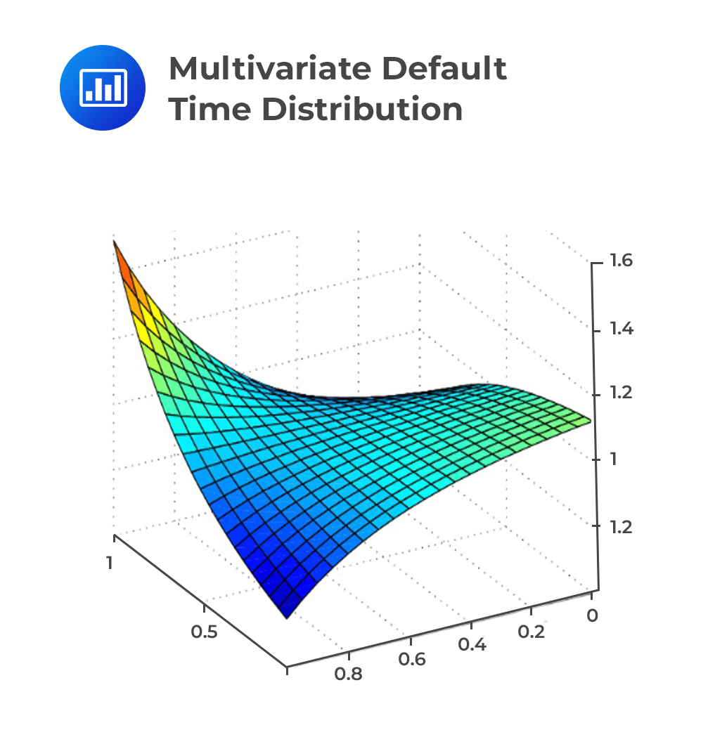So, how do copulas come in? Let’s assume that we have a portfolio with securities n of issuers and have estimated single issuer default-time distributions F1(t1) , . . . , Fn(tn). Since we do not know the joint distribution F(t1, …tn), we specify a copula function \(\text{c}\left( \text{F}\left( \text{t1},…,\text{tn} \right) \right)\), specifying that:

$$ \text{c}\left( \text{F}\left( \text{t1},…,\text{tn} \right) \right) =\text{F}\left( \text{t1},…,\text{tn} \right) $$

In a summary, there are four steps in computing a credit VaR:

1. Specify the copula function that will be used.
2. Simulate the default times.
3. Apply the default times to the portfolio to get the market values and P&Ls in each possible scenario.
4. Add the result to get portfolio distribution statistic.

Granularity and Portfolio Credit Value-at-Risk

Portfolio Credit VaR is similar to the VAR of a single VaR and it is defined as a quantile of the credit loss, minus the expected loss of a portfolio. 

Default correlation significantly affects portfolio risk. However, it impacts the volatility and extreme quantiles of loss rather than the expected loss. If the default correlation in a portfolio of credits is equal to 1, then the portfolio behaves as if it comprises just one credit. As such, there is no credit diversification. On the other hand, if the default correlation is equal to 0, then the number of defaults in the portfolio is a random variable with a binomial distribution. As such,  there is considerable credit diversification.

Effect of Granularity on Credit VaR

We should consider what happens when a portfolio becomes more granular, i.e., if it consists of more independent credits, each of which is a smaller fraction of the portfolio. 

In general, a portfolio with a higher probability of default has a higher Credit VaR. Credit VaR decreases, however, as the granularity of the portfolio increases for a given default probability. When the default probability is high, convergence is even more pronounced. There is an important flip-side to this: If the default probability is low, it is harder to reduce VaR by making the portfolio more granular.  

Eventually, for a portfolio with many small credit positions, probability will converge at 100%, which means that the credit loss will equal the expected loss. The single-credit portfolio experiences no loss with probability \(1 – \lambda\), and total loss with probability \(\lambda\), while the granular portfolio experiences a loss of \(100 \lambda\)% “almost surely.” The portfolio then experiences no volatility of credit loss, and the Credit VaR is zero.  

Practice Question

The conditional cumulative probability of default by a single credit is given by \(\emptyset \left( 3.254 \right) =0.1124\).What is the default threshold if \({ \beta }_{ i }=0.74\) and \(m=0.586\) ?

A. 2.6223.

B. 0.5092.

C. 2.1887.

D. 3.2154.

The correct answer is A.

The conditional cumulative default probability function can be given as:

$$ p\left( m \right) =\emptyset \left( \frac { { k }_{ i }-{ \beta }_{ i }{ m } }{ \sqrt { 1-{ \beta }_{ i }^{ 2 } } } \right) $$

From the problem,we have: \({ \beta }_{ i }=0.74\) and \(m=0.586\). We have to solve for \({ k }_{ i }\).

Therefore:

$$\begin{align*} \emptyset \left( 2.56 \right) =\emptyset \left( \frac { { k }_{ i }-{ \beta }_{ i }{ m } }{ \sqrt { 1-{ \beta }_{ i }^{ 2 } } } \right) &=0.1124\\  \Rightarrow \left( \frac { { k }_{ i }-0.74\times 0.586 }{ \sqrt { 1-{ 0.74 }^{ 2 } } } \right) &=3.254\\ \Rightarrow { k }_{ i }-0.74\times 0.586&=3.254\times \sqrt { 1-{ 0.74 }^{ 2 } }\\ \Rightarrow { k }_{ i }&=3.254\times \sqrt { 1-{ 0.74 }^{ 2 } } +0.74\times 0.586\\ &=2.6223 \end{align*}$$