Modern Portfolio Theory (MPT) and the Capital Asset Pricing Model (CAPM)

After completing this reading, you should be able to:

• Explain modern portfolio theory and interpret the Markowitz efficient frontier.
• Understand the derivation and components of the CAPM.
• Describe the assumptions underlying the CAPM.
• Interpret and compare the capital market line and the security market line.
• Apply the CAPM in calculating the expected return on an asset.
• Interpret beta and calculate the beta of a single asset or portfolio.
• Calculate, compare, and interpret the following performance measures: the Sharpe performance index, the Treynor performance index, the Jensen performance index, the tracking error, information ratio, and the Sortino ratio.

Exam tip: Be sure to understand the calculations behind the CAPM because there is a strong likelihood you will be getting mathematical questions on this in your FRM part 1 exam.

Modern Portfolio Theory

Modern portfolio theory is attributed to Harry Markowitz, who postulated that a rational investor should evaluate the potential portfolio allocations based on means and variances of the expected return distributions.

Assumptions of the Modern Portfolio Theory

I. The capital markets are perfect. Perfect market implies that:

• There are no transaction costs and taxes.
• All market participants can access available information without any cost.
• There is perfect competition in the market.

II. The returns from the portfolios are normally distributed. This allows the characteristics of the returns to be stated in terms of the mean and the variance.

Markowitz suggested that the size of investment made by an institution should be based on the contribution of the assets to the entire portfolio’s return (in terms of mean and return). The assets’ performance is not evaluated independently but rather with the performance of other assets.

Portfolio diversification is one method of decreasing the risk exposure to each asset. Thus, investors must be compensated for accepting the risk in each asset.   Diversification enables the maximization of the level of returns at any provided level of risk.

Markowitz Efficient Frontier

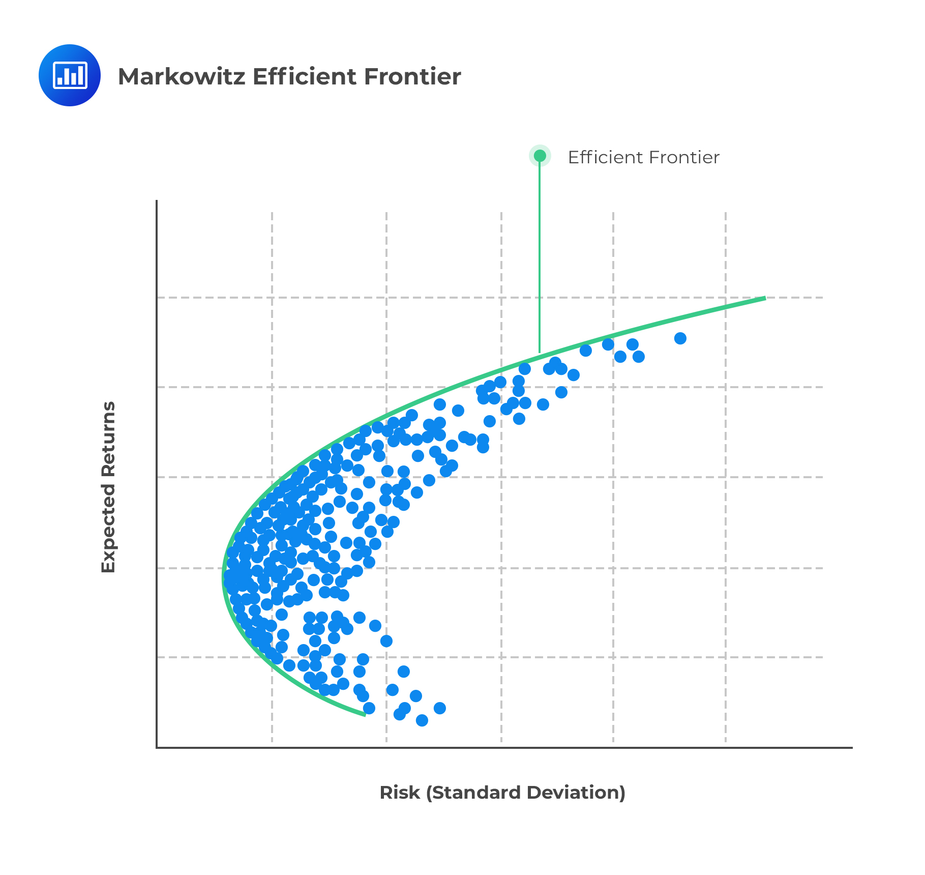
The Markowitz Efficient Frontier (or only efficient frontier) is a curved solid curve with a plot of the optimal returns for each level of risk. Each point on the curve represents the maximum level of portfolio return for a given level of risk.

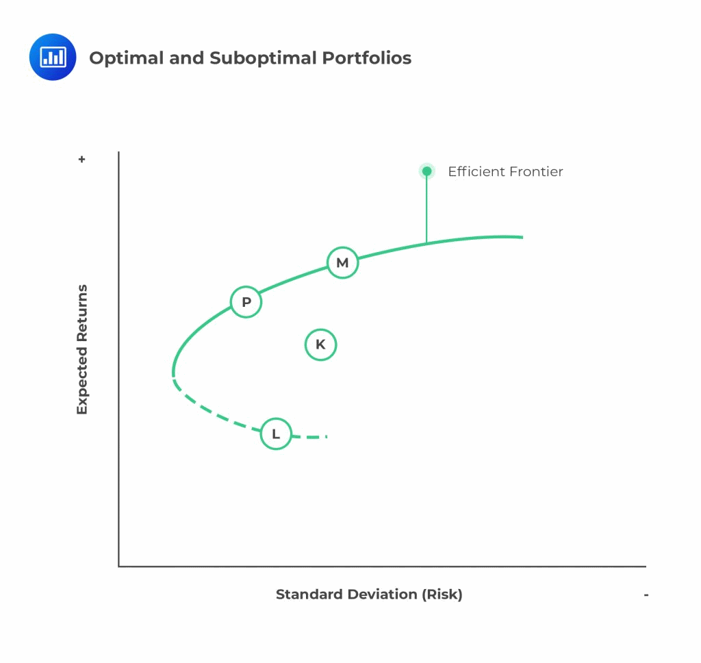
Now, consider the following efficient frontier.

Portfolio P gives the best return for the same level of risk. On the other hand, portfolio K is termed as suboptimal since there are other portfolios (located on the vertical distance between the portfolio K and the efficient frontiers) that can offer better returns for the same level of risk, namely portfolio M.

Portfolio M is referred to as the market portfolio. The market portfolio assumes that the market attains the equilibrium and appropriately includes all the risky assets in the economy weighted by their respective market values.

Portfolio P is also an efficient portfolio but representing a lower level of risk than portfolio M.

From the efficient frontier, it is easy to see that the expected return is increased by increasing the portfolio’s risk level and vice versa. The dotted line represents the most inefficient portfolios; in this case, portfolio L. Inefficient portfolios imply that the investor achieves the lowest level of return given any level of risk.

The Capital Asset Pricing Model (CAPM)

The Capital Asset Pricing Model, derived by Sharpe, Lintner, and Mossin, stipulates assumptions regarding the market and how investors behave to enable the creation of an equilibrium model of prices in the whole market. CAPM explains that the market equilibrium is attained when all investors hold portfolios whose constituents are a combination of riskless assets and the market portfolio.

Assumptions Underlying the CAPM

Assumptions of the CAPM model include:

• There are no transaction costs
• There are no taxes
• Assets are infinitely divisible
• Unlimited short-selling is permissible
• All assets are marketable/liquid
• Investors are price takers whose individual buy and sell transactions do not affect the price
• Investors’ utility functions are based solely on expected portfolio return and risk
• The only concern among investors are risk and return over a single period, and the single period is the same for all investors.

Under these assumptions, the expected rate of return over a given holding time is given by:

$$ E\left( { R }_{ i } \right) ={ R }_{ f }+{\beta}_i \left( { R }_{ m }-{ R }_{ f } \right) $$

Where

\(E(R_i )\): the expected return of asset i over the holding period

\(R_f\): rate of return on the risk-free asset

\(R_m\): Expected market return over the holding period

\(β_i\): the Beta factor of the asset i

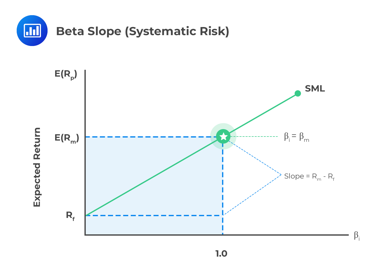
Note that \(\left( { R }_{ m }-{ R }_{ f } \right)\) is the expected return per unit risk (beta) and \({\beta}_i \left( { R }_{ m }-{ R }_{ f } \right)\) is the expected return above the risk-free rate of return.

Interpreting Beta

Beta is a measure of the systematic risk associated with a particular stock, asset, or portfolio. Systematic risk is the portion of risk that cannot be eliminated by any amount of diversification.

A value of beta above 1 indicates a stock/asset/portfolio that has, historically, amplified the return of the whole market (positive or negative). A beta close to zero would indicate a stock/asset/portfolio that provides a more stable return than the market as a whole. A negative beta would signify a stock/asset/portfolio whose performance is counter-cyclical, i.e., offsets the overall market experience.

For company \(i\):

$${\beta}_{i}=\frac{Cov(i,m)}{{\sigma}_{m}^{2}}=\frac {{\sigma}_{im}}{ {\sigma}_{m}^{2}} $$

Where \({ \sigma }_{ m }\) is the variance of the market index and \({ \sigma }_{ im }\) the covariance between the individual stock’s/asset’s return and that of the market.

Alternatively, by using the fact that:

$$Corr(i,m)={\rho}_{im}=\frac{Cov(i,m)}{{\sigma }_{ i }{\sigma}_{ m }}=\frac{{\sigma}_{im}}{{ \sigma }_{ i }{ \sigma }_{ m }}$$

$$\Rightarrow { \sigma }_{im}={\rho}_{im}.{ \sigma }_{ i }{ \sigma }_{ m }$$

We can write:

$$ { \beta }_{ i }={ \rho }_{ im }\frac { { \sigma }_{ i } }{ { \sigma }_{ m } } $$

Where

\(ρ_{im}\): correlation coefficient between returns of asset i and that of the market portfolio.

\(σ_i\): standard deviation of asset i

\(σ_m\): standard deviation of the market portfolio

Therefore, we can write:

$$E(R_i) = R_f +{\sigma}_{i} {\rho}_{im} \left(\frac{R_m – R_f}{{\sigma}_{m}}\right)$$

This is the equation of the security market line (SML). The equation implies that the expected return on any asset is equivalent to a risk-free rate of return plus the premium. The SML implies that the expected return on any asset can be expressed as the linear function of assets covariance with the whole market.

Derivation of CAPM

The derivation of CAPM involves three major steps:

1. Recognize that investors are only compensated for bearing systematic risk, not specific risks that can easily be diversified away. Note that, beta is an appropriate measure of systematic risk.
2. Suppose we recognize that portfolio expected return is a weighted average of individual expected returns and portfolio beta is a weighted average of the individual betas. In that case, we can show that portfolio return is a linear function of portfolio beta. And because arbitrage prevents mispricing of assets relative to systematic risk, then an individual asset’s expected return is a linear function of its beta.
3. We can then use the risk-free asset and the market portfolio to solve for the intercept and slope of the CAPM.

$$ E\left( { R }_{ i } \right) ={ R }_{ f }+\beta \left( { R }_{ m }-{ R }_{ f } \right) $$

The Capital Market Line

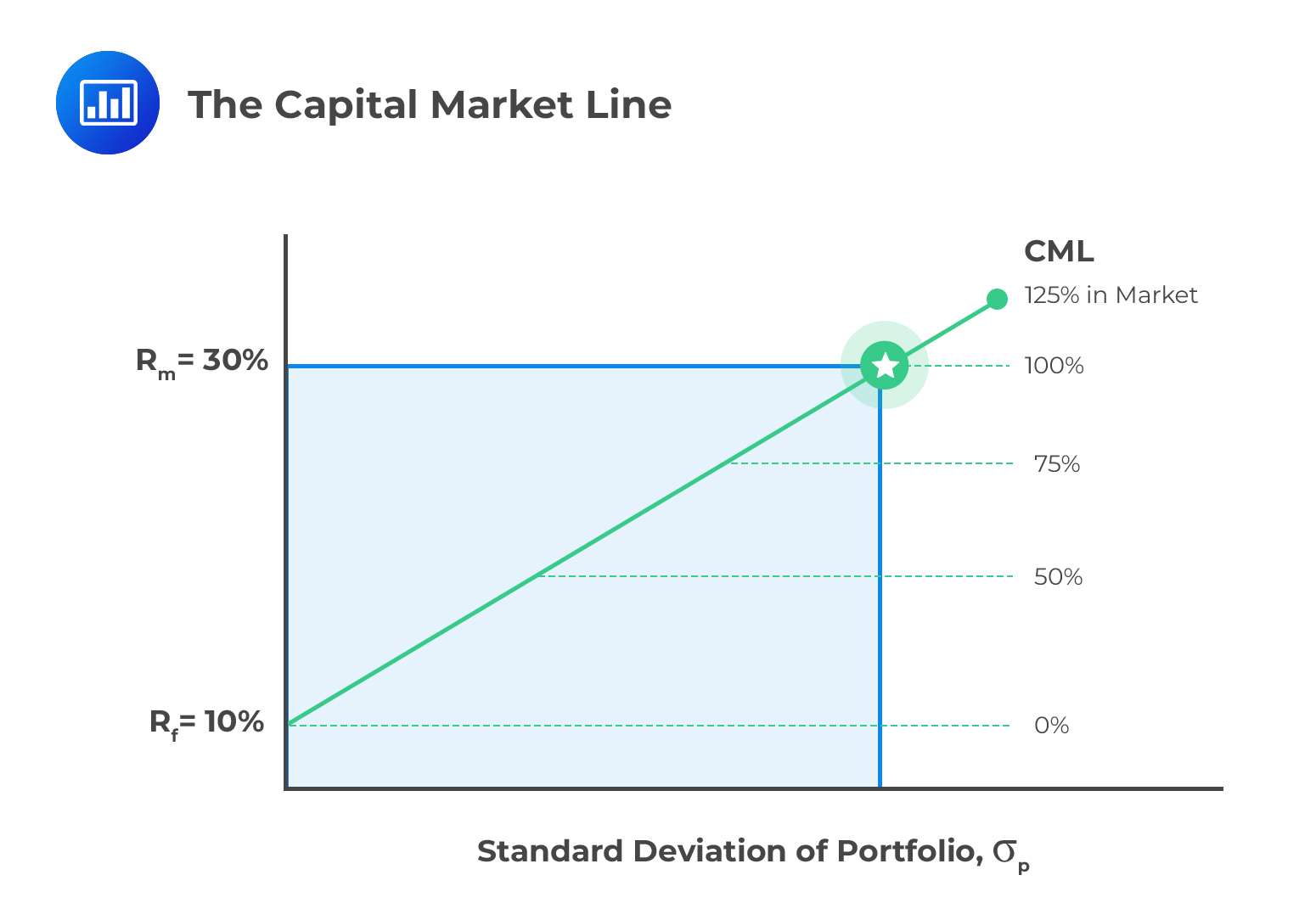
The capital market line expresses the expected return of a portfolio as a linear function of the risk- free rate, the portfolio’s standard deviation, and the market portfolio’s return and standard deviation.

$$ E\left( { R }_{ C } \right) ={ R }_{ f }+\left[ \frac { E\left( { R }_{ m } \right) -{ R }_{ f } }{ { \sigma }_{ m } } \right] { \sigma }_{ C } $$

Where

\(E(R_C)\) is the expected return of any portfolio on the efficient frontier

\(σ_C\) is the standard deviation of the return on portfolio C

\(E(R_m )\)   is  the expected return on the market portfolio

\(σ_m\) is the standard deviation of the return on the market portfolio

\(R_f\) is the risk-free rate of return.

The capital market return implies that the return on any portfolio is a linear function of its standard deviation. The variable \(\left[ \frac { E\left( { R }_{ m } \right) -{ R }_{ f } }{ { \sigma }_{ m } } \right]\) is termed as the market price of risk or the risk premium.

Single-Index Performance Measurement Indicators

The Sharpe Performance Index (SPI)

The Sharpe ratio is equal to the risk premium divided by the standard deviation:

$$SPI=\frac { E\left( { R }_{ p } \right) -{ R }_{ f } }{ \sigma \left( { R }_{ P } \right) } $$

Where:

\(E\left( { R }_{ p } \right)\) = portfolio’s expected return

\({ R }_{ f }\) = risk-free rate

\(\sigma \left( { R }_{ P } \right)\) = standard deviation of returns of the portfolio

The Sharpe ratio, or reward-to-variability ratio, is the slope of the capital allocation line (CAL). The greater the slope (higher number), the better the asset. Note that the risk being used is the total risk of the portfolio, not its systematic risk, which is a limitation of the measure. The portfolio with the highest Sharpe ratio has the best performance, but the Sharpe ratio by itself is not informative. In order to rank portfolios, the Sharpe ratio for each portfolio must be computed.

A further limitation occurs when the numerators are negative. In this instance, the Sharpe ratio will be less negative for a riskier portfolio resulting in incorrect rankings.

The Treynor Performance Index (TPI)

The Treynor measure (1965) of a portfolio is explained by the expression below.

$$ TPI=\frac { E\left( { R }_{ p } \right) -{ R }_{ f } }{ { \beta }_{ p } } $$

Where:

\(E\left( { R }_{ p } \right)\) = portfolio’s expected return

\({ R }_{ f }\) = risk-free rate

\({ \beta }_{ p }\) = beta of the portfolio

Treynor measures the risk premium per unit risk (Beta). As with the Sharpe ratio, the Treynor ratio requires positive numerators to give meaningful comparative results and the Treynor ratio does not work for negative beta assets. Also, while both the Sharpe and Treynor ratios can rank portfolios, they do not provide information on whether the portfolios are better than the market portfolio or information about the degree of superiority of a higher ratio portfolio over a lower ratio portfolio.

The Jensen Performance Index (JPI)

Jensen’s alpha (Jensen, 1968) is described as an asset’s excess return over and above the return predicted by CAPM.

$$ \text{ Jensen’s measure of a portfolio }={ \alpha }_{ p }=E\left( { R }_{ p } \right) -\left[ { R }_{ f }+{ \beta }_{ p }\left( E\left( { R }_{ m } \right) -{ R }_{ f } \right) \right] $$

Jensen’s alpha is based on systematic risk. The daily returns of the portfolio are regressed against the daily market returns to compute a measure of this systematic risk in the same manner as the CAPM. The difference between the actual return of the portfolio and the calculated or modeled risk-adjusted return is a measure of performance relative to the market.

If αp is positive, the portfolio has outperformed the market, whereas a negative value indicates underperformance. The values of alpha can be used to rank portfolios or the managers of those portfolios, with the alpha being a representation of the maximum an investor should pay for the active management of that portfolio.

Relationships Between Treynor and Jensen Performance Indices

Denote the JPI by \({ \alpha }_{ p }\) which is the y-intercept of the regression equation:

$$E\left(R_p\right)-R_f ={ \alpha }_{ p }+{ \beta }_{ p }\left(E\left(R_m\right)-R_f\right)$$

Divide the equation above by \({ \beta }_{ p }\) to get:

$$\frac{E\left(R_p\right)-R_f}{{ \beta }_{ p }}=\frac{{ \alpha }_{ p }}{{ \beta }_{ p }} +\left(E\left(R_m\right)-R_f\right)$$

The left-hand side of the equation above is just TPI. So,

$$\text{Treynor Performance Index}=TPI=\frac{{ \alpha }_{ p }}{{ \beta }_{ p }} +\left(E\left(R_m\right)-R_f\right)$$

For a greater performance, \(TPI>E\left(R_m\right)-R_f\)  and thus  \(\frac{α_p}{β_p} >0\). Also, \(β_p>0\) for almost all assets and thus it must be true that \(α_p>0\). From these results is evident to say that if a superior performance is demonstrated by TPI, then is also the case for JPI and vice versa.

The Tracking Error (TE)

Tracking error measures the difference between a portfolio’s return and that of a benchmark level, which was meant to be surpassed by the tracking error. We need to calculate the quantity:

$$ TE= \left( { R }_{ P }-{ R }_{ B } \right) $$

Where

\(R_P\): the return of the portfolio is considered

\(R_B\): Return on the benchmark portfolio

Another way of calculating the TE is to calculate the standard deviation of the difference in the portfolio and the benchmark return:

$$TE=\sqrt{\frac{\sum{(R_P-R_B)^2}}{N-1}}$$

Where N is the number of periods under consideration.

The Information Ratio (IR)

The information ratio is similar to SPI, only that it is the active return relative to the benchmark portfolio divided by the standard deviation of the active return \(\left(R_P-R_B\right)\):

$$ IR=\frac{E(R_P-R_B)}{\sqrt{Var (R_P-R_B)}}$$

Where:

\({ R }_{ P }\)=portfolio return and

\({ R }_{ B }\)=benchmark return

IR can be used in place of TE

The Sortino Ratio (SR)

The Sortino ratio is much like the Sharpe ratio, but there are two glaring differences:

• The risk-free rate is replaced with a minimum acceptable return, denoted as \({ R }_{ min }\)
• The standard deviation is replaced by a semi-standard deviation, which measures the variability of only those returns that fall below the minimum acceptable performance.

The measure of risk is the square root of the mean squared deviation from T of those observations in period t where \(T > R_{Pt}\), else zero.

$$SR=\frac{(E(R_P )-T}{\sqrt{\frac{1}{N}\sum_{t=1}^{N}{min(0,R_{Pt} -T)^2}}}$$

Where T is the target or required rate of return (which can be a risk-free rate or any other rate) for an investment decision. It is also termed as the minimum acceptable rate of return (MAR).

Question 

Alpha Investments uses the Markowitz efficient frontier to optimize client portfolios. The efficient frontier plots risk vs. expected returns for various portfolio combinations.

Which if the following statements is most likely correct?

A. Portfolios located above the efficient frontier provide the highest returns for a given level of risk.

B. Portfolios located below the efficient frontier are the most optimal as they offer lower risk for the same level of return.

C. The efficient frontier illustrates the relationship between risk and return for individual assets rather than portfolios.

D. Any portfolio on the efficient frontier offers either the highest return for a given level of risk or the lowest risk for a targeted level of return.

Solution

The correct answer is D.

The Markowitz efficient frontier represents the set of optimal portfolios that achieve the best trade-off between risk and return. Portfolios located on the efficient frontier offer either the highest possible return for a given level of risk or the lowest possible risk for a targeted level of return. Investors aim to construct portfolios on the efficient frontier to achieve the best risk-return trade-off and maximize their investment outcomes.

A is incorrect because portfolios located above the efficient frontier are considered inefficient, offering higher risk for the same level of returns, and therefore, they do not provide the highest returns for a given level of risk.

B is incorrect because portfolios located below the efficient frontier are considered suboptimal as they offer lower returns for the same level of risk, and thus, they are not the most optimal.

C is incorrect because the efficient frontier does not illustrate the relationship between risk and return for individual assets. Instead, it represents the risk-return relationship for portfolios constructed by combining different assets.

Things to Remember

• Efficient portfolios are considered optimal choices as they provide the best risk-return trade-off among all possible portfolios.
• Portfolios above the efficient frontier are inefficient since they have higher risk without offering higher returns, while portfolios below the efficient frontier are also suboptimal, providing lower returns for the same level of risk.
• The efficient frontier primarily represents diversified portfolios, where different assets are combined to achieve varying risk-return profiles.