


Corporate Bonds
After completing this reading, you should be able to: Understand what a bond... Read More

After completing this reading you should be able to:
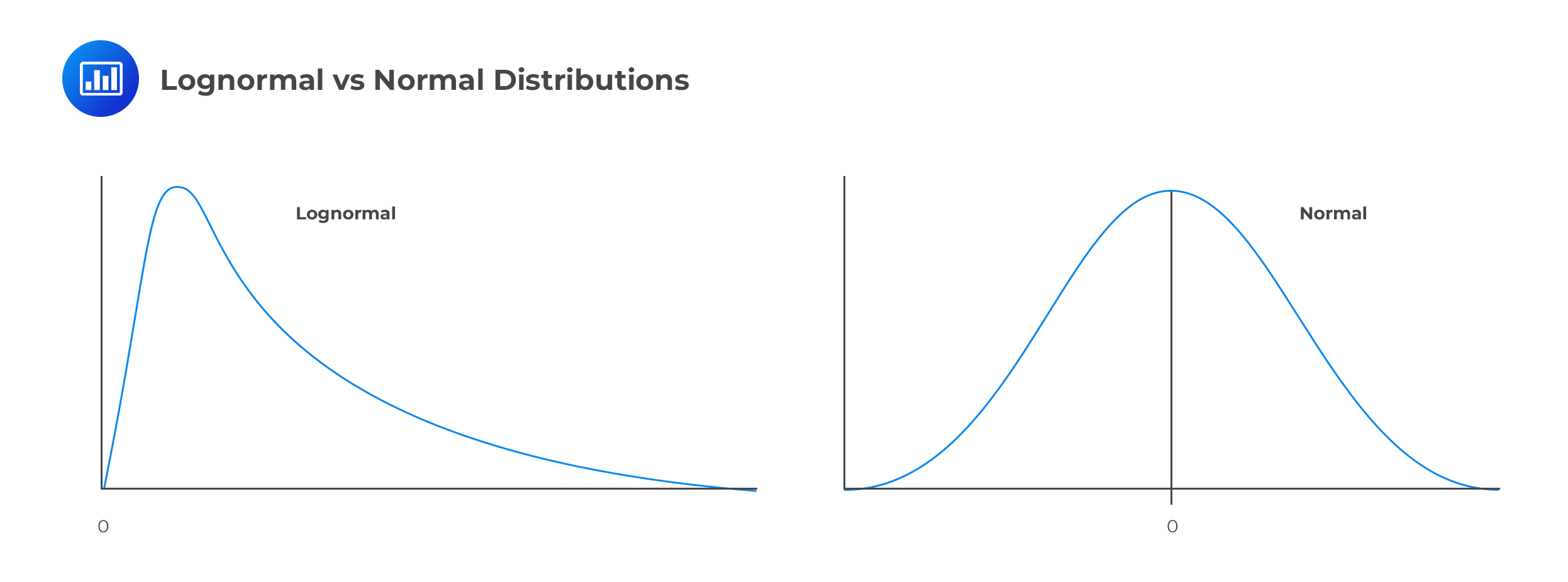
Suppose we have a random variable X. This variable will have a lognormal distribution if its natural log (ln X) is normally distributed. In other words, when the natural logarithm of a random variable is normally distributed, then the variable itself will have a lognormal distribution.
The two most essential characteristics of the lognormal distribution are as follows:
These characteristics are in direct contrast to those of the normal distribution, which is symmetrical (zero-skew) and can take on both negative and positive values. As a result, the normal distribution cannot be used to model stock prices because stock prices cannot fall below zero. The lognormal distribution is also used to value options.
 The Lognormal Property of Stock Prices
A crucial part of the BSM model is that it assumes stock prices are log-normally distributed. Precisely,
$$ \text{ln}{ \text{S} }_{ \text{T} }\sim \text{N}\left( \text{ln}{ \text{S} }_{ 0 }+\left( \mu -\cfrac { { \sigma }^{ 2 } }{ 2 } \right) \text{T},{ \sigma }^{ 2 }\text{T} \right) $$
Where:
\({\text{S}}_{\text{T}}\)=stock price at time T
\({\text{S}}_{\text{0}}\)=stock price at time 0
\(\mu \)=expected return on stock per year
\(\sigma \)=annual volatility of the stock price
Note: The above relationship holds because mathematically, if the natural logarithm of a random variable \(x\), ln(\(x\)) is normally distributed, then \(x\) has a lognormal distribution. It’s also imperative to note that the BSM model assumes stock prices are lognormally distributed, with stock returns being normally distributed. Specifically, continuously compounded annual returns are normally distributed with a mean of \(\text{ln}{ \text{S} }_{ \text{0} }+\left[ \mu -\frac{ { \sigma }^{ 2 } }{ 2 } \right]\) and a variance of \(\sigma^{ 2 }T\).
ABC stock has an initial price of $60, an expected annual return of 10%, and annual volatility of 15%. Calculate the mean and the standard deviation of the distribution of the stock price in six months.
$$ \begin{align*} & \text{ln}{ \text{S} }_{\text{T}} \sim \text{N}\left( \text{ln}{ \text{S} }_{ 0 }+\left( \mu -\cfrac { { \sigma }^{ 2 } }{ 2 } \right) \text{T},{ \sigma }^{2}{ \text{T} } \right) \\\Rightarrow &\text{ln}{ \text{S} }_{\text{T}} \sim \text{N}\left[ \text{ln}60+\left( 0.10-\cfrac { { 0.15 }^{ 2 } }{ 2 } \right) 0.5,{ 0.15 }^{ 2 }\times 0.5 \right] \\& \Rightarrow \text{ln}{ \text{S}}_\text{T}\sim \text{N}\left[ 4.1387, 0.01125 \right] \end{align*} $$
In this case, the standard deviation of the distribution of the stock price is \(\sqrt{0.01125}=0.1061\)
Sometimes, the Global Association of Risk Professionals (GARP) may want to test your understanding of the lognormal concept by involving confidence intervals. Since \(\text{lnS}_{\text T}\) is log-normally distributed, 95% of values will fall within 1.96 standard deviations of the mean. Similarly, 99% of the values will fall within 2.58 standard deviations of the mean. For example, to obtain the 99% confidence interval for stock prices using the above data, we will proceed as follows:
From the above calculations, we have, \(\text{ln}{ \text{S}}_{\text{T}} \sim \text{N}\left[ 4.1387,0.01125 \right]\)
To find the two-sided confidence interval at 99% confidence level, we apply the formula:
$$\text{ln}{ \text{S}}_{\text{T}}=\mu \pm { \text{z} }_{ \alpha }\times \text{SD}$$
Note that, in this case, \(\text{SD}=\sqrt{0.01125}=0.1061\).
$$\begin{align*}
4.1387 – z_{\alpha} \times \text{SD} &< \ln S_T < 4.1387 + z_{\alpha} \times \text{SD} \\
e^{4.1387 – z_{\alpha} \times \text{SD}} &< S_T < e^{4.1387 + z_{\alpha} \times \text{SD}} \\47.70 &< S_T < 82.47 \end{align*}$$
Using the properties of a lognormal distribution, we can show that the expected value of \({\text{S}}_{\text{T}}, {\text{E}}({\text{S}}_{\text{T}} )\), is:
$$ {\text{E}}({\text{S}}_{\text{T}} )={ \text{S} }_{ 0 }{ \text{e} }^{ \mu \text{T} } $$
\(\mu\)=expected rate of return
The current price of a stock is $40, with an expected annual return of 15%. What is the expected value of the stock in six months?
$$ \text{Expected stock price}={$40}{ \text{e} }^{ 0.15 \times 0.5}=$43.11 $$
$$ \text{R}_{ \text{pr} }={ \left[ { \text{r} }_{ 1 }\times { \text{r} }_{ 2 }\times { \text{r} }_{ 3 }\times \cdots \times { \text{r} }_{ \text{n} } \right] }^{ \cfrac { 1 }{ \text{n} } }-1 $$
\({\text{r}}_{\text{i}}\)=portfolio return at the time i
The continuously compounded return realized over some time of length T is given by:
$$ { \cfrac { 1 }{ \text{T} } \text{ln}\left( \cfrac { { \text{S} }_{ \text{T} } }{ { \text{S} }_{ 0 } } \right) } $$
The realized return of a stock initially priced at $50 growing, with volatility, to $87 over five periods would simply be:
$$ \text{Realized return }={ \cfrac { 1 }{5} \text{ln}\left( \cfrac { $87 }{ $50 } \right) }=11.08\% $$
We can calculate historical volatility from daily price data of stock. We simply need to calculate continuously compounded returns per day and then determine the standard deviation.
The continuously compounded return for the day i is calculated as:
$$ \text{ln}\left( \cfrac { { \text{S} }_{ \text{i} } }{ { \text{S} }_{ \text{i}-1 } } \right) $$
The volatility of short periods can be scaled to give the volatility of more extended periods.
For example,
$$ \text{Annual volatility }=\text{daily volatility }\times \sqrt{(\text{ no.of trading days in a year})} $$
Note that this formula is useful throughout the whole FRM part 1 and FRM part 2 exams in estimating volatility.
Conversely,
$$ \text{daily volatility }=\cfrac { \text{annual volatility} }{ \sqrt{\text{ no.of trading days in a year} } } $$
The Black-Scholes-Merton model is used to price European options and is undoubtedly the most critical tool for the analysis of derivatives. It is a product of Fischer Black, Myron Scholes, and Robert Merton.
The model takes into account the fact that the investor has the option of investing in an asset earning the risk-free interest rate. The overriding argument is that the option price is purely a function of the volatility of the stock’s price (option premium increases as volatility increases).
The value of a call option is given by:
$$ { \text{C} }_{ 0 }={ \text{S} }_{ 0 }\times \text{N}\left( { \text{d} }_{ 1 } \right) -\text{K}{ \text{e} }^{ -\text{rT} }\times \text{N}\left( { \text{d} }_{ 2 } \right) $$
The value of a put option is given by:
$$ \text{P}_{ 0 }=\text{K}{ \text{e} }^{ -\text{rT} }\times \text{N}\left( { -\text{d} }_{ 2 } \right) -{ \text{S} }_{ 0 }\times \text{N}\left( -{ \text{d} }_{ 1 } \right) $$
Where:
$$ \begin{align*} { \text{d} }_{ 1 }&=\cfrac { \text{ln}\left( \cfrac { { \text{S} }_{ 0 } }{ \text{K} } \right) +\left[ \text{r}+\left( \cfrac { { \sigma }^{ 2 } }{ 2 } \right) \right] \text{T} }{ \sigma \sqrt { \text{T} } } \\ { \text{d} }_{ 2 }&={ \text{d} }_{ 1 }-\left({ \sigma \sqrt { \text{T} } }\right) \end{align*} $$
T =time to maturity,assuming 365 days per year
\({\text{S}}_{0}\)=asset price
K =exercise price
\({\text{R}}_{\text{f}}^{\text{c}}\)=continuously compounded risk-free rate
\(\sigma\)=volatility of continuously compounded returns on the stock
\(\text{N}({\text{d}}_{\text{i}}) \)=cumulative distribution function for a standardized normal distribution variable
Assume \({\text{S}}_{0}\) = $100, K = $90, T = 6 months, r = 10%, and \(\sigma\) = 25%.
Calculate the value of a call option.
$$ \begin{align*} { \text{d} }_{ 1 }&=\cfrac { \text{ln}\left( \cfrac { { \text{S} }_{ 0 } }{ \text{K} } \right) +\left[ \text{r}+\left( \cfrac { { \sigma }^{ 2 } }{ 2 } \right) \right] \text{T} }{ \sigma \sqrt { \text{T} } } \\ &=\cfrac { \text{ln}\left( \cfrac { 100 }{ 90 } \right) +\left[ 0.10+\left( \cfrac { { 0.25 }^{ 2 } }{ 2 } \right) \right] 0.5 }{ 0.25\sqrt { 0.5 } } =\cfrac { 0.1053+0.0656 }{ 0.1768 } =0.9672 \\ \text d_2 & =\text d_1-(\sigma \sqrt{\text T})=0.9672-(0.25 \sqrt{0.5}) =0.7904 \\ \end{align*} $$
From a standard normal probability table, look up N(0.97) = 0.8333 and N(0.79) = 0.7852.
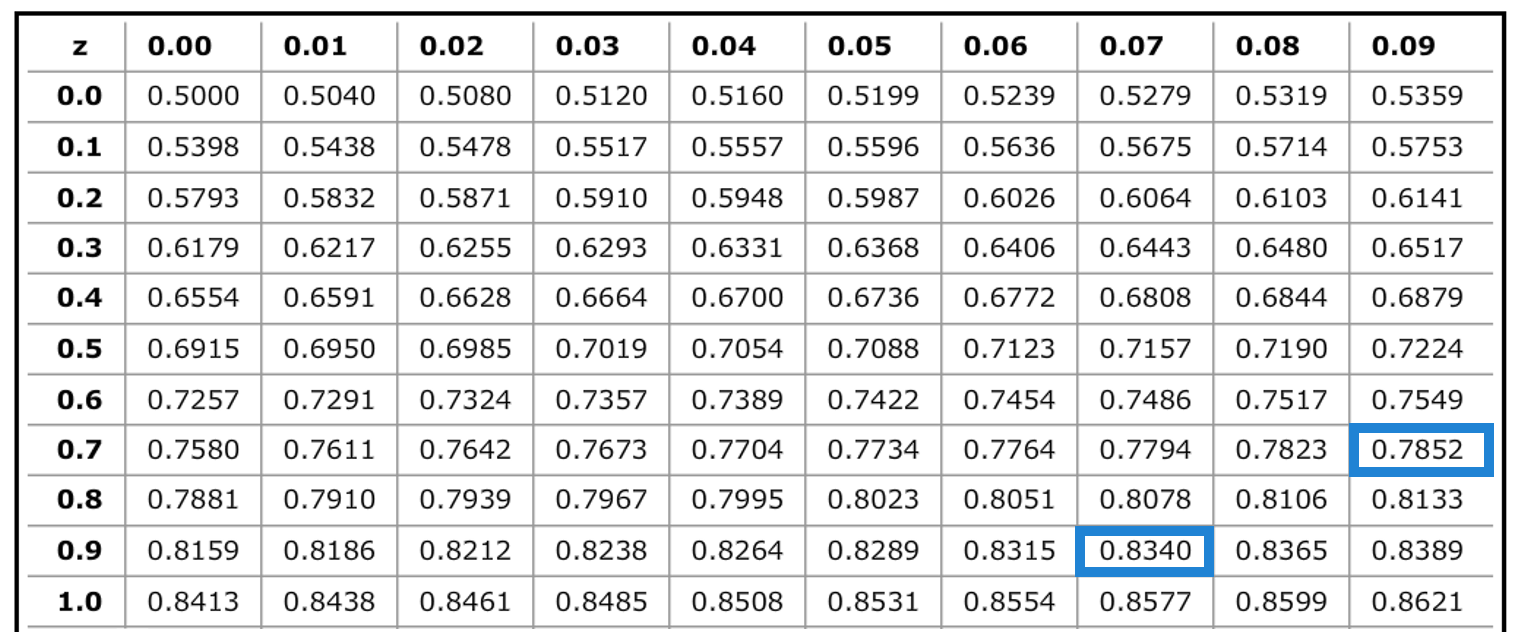
$$ \begin{align*} { \text{C} }_{ 0 }&={ \text{S} }_{ 0 }\times \text{N}\left( { \text{d} }_{ 1 } \right) -\text{K}{ \text{e} }^{ -\text{rT} }\times \text{N}\left( { \text{d} }_{ 2 } \right) \\ &=100\times \text N\left( 0.8340 \right) -90{\text e }^{ -0.10 \times 0.50 }\times \text N\left( 0.7852 \right) =$16.17 \end{align*} $$
Note that the intrinsic value of the option is $10—our answer must be at least that amount.
Tip 1: Given one of either the put value or the call value, you can use the put-call parity to find the other. Precisely,
$$ \begin{align*} { \text{C} }_{ 0 }&=\text{P}_{ 0 }+{ \text{S} }_{ 0 }-\left( \text{K}{ \text{e} }^{ \left( -{ { \text{R} } }_{ { \text{f} } }^{ { \text{c} } }\text{T} \right) } \right) \\ { \text{P} }_{ 0 }&=\text{C}_{ 0 }-{ \text{S} }_{ 0 }+\left( \text{K}{ \text{e} }^{ \left( -{ { \text{R} } }_{ { \text{f} } }^{ { \text{c} } }\text{T} \right) } \right) \end{align*} $$
Tip 2: \(\text{N}(−\text{d}_\text{1})=1−\text{N}(\text{d}_\text{1})\)
Tip 3: As \(\text S_0\) becomes very large, calls (puts) are extremely in-the-money (out-of-the-money)
Tip 4: As \({\text{S}}_{0}\) becomes very small, calls (puts) are extremely out-of-the-money (in-the-money)
Tip 5: Although \(\text{N}(−\text{d}_\text{1})\)and \(\text{N}(−\text{d}_{2})\) can easily be identified from statistical tables; sometimes you’ll be asked to compute \(\text{d}_{2}\) and \(\text{d}_{2}\) without the formulas.
Assume that we have a known dividend d distributed a time \({\text{T}}_{\text{1}},{\text{T1}} < {\text{T}}\) where T is the maturity date. To value calls and puts when there are such dividends, we modify the BSM model by replacing \({\text{S}}_{\text{0}}\)withS, where:
$$ \text{S}={\text{S}}_{0}-{\text{D}} $$
D is the sum of the PV(discounted at \({ { \text{R} } }_{ { \text{f} } }^{ { \text{c} } }\) ) of the dividend payments during the life of the option.
$$ \begin{align*} \text{ For example,with dividends } \text{D}_{1} \text{ and } \text{D}_{2} \text{ at times } {\Delta}\text{t}_{1} \text{ nd } { \Delta}\text{t}_{2}, \\ \text{S}={ \text{S} }_{ 0 }-{ \text{D} }_{ 1 }{ \text{e} }^{ -\left( { { \text{R} } }_{ { \text{f} } }^{ { \text{c} } } \right) \cfrac { \Delta { \text{t} }_{ 1 } }{ \text{m} } }-{ \text{D} }_{ 2 }{ \text{e} }^{ -\left( { { \text{R} } }_{ { \text{f} } }^{ { \text{c} } } \right) \cfrac { \Delta { \text{t} }_{ 2 } }{ \text{m} } } \end{align*} $$
\({\Delta }{\text{t}}_{\text{i}}\) represents the amount of time until the ex-dividend date
m a division factor in bringing the \(\Delta t\) to a full year. e.g. \(\Delta t=2\Delta t=2\) months, m=12 months, so \( \cfrac { \Delta { \text{t} }_{ 1 } }{ \text{m} } =\cfrac {2}{12}=0.1667\) years .
After this, everything else in the computational formulas remains the same, i.e.,
The value of a call option is given by:
$$ { \text{C} }_{ 0 }=\left[ { \text{S} }_{ 0 }\times \text{N}\left( { \text{d} }_{ 1 } \right) \right] -\left| \text{K}\times { \text{e} }^{ \left( -{ { \text{R} } }_{ { \text{f} } }^{ { \text{c} } }\times \text{T} \right) }\times \text{N}\left( { \text{d} }_{ 2 } \right) \right| $$
The value of a put option is given by:
$$ \begin{align*} \text{P}_{ 0 }&=\left[ \text{K}\times { \text{e} }^{ \left( -{ { \text{R} } }_{ { \text{f} } }^{ { \text{c} } }\times \text{T} \right) }\times \left( 1-\text{N}\left( { \text{d} }_{ 2 } \right) \right) \right] -\left[ \text{S}\times \left( 1-\text{N}\left( { \text{d} }_{ 1 } \right) \right) \right] \\ { \text{d} }_{ 1 }&=\cfrac { \text{ln}\left( \cfrac { { \text{S} } }{ \text{K} } \right) +\left[ { { \text{R} } }_{ { \text{f} } }^{ { \text{c} } }+\left( 0.5\times { \sigma }^{ 2 } \right) \right] \text{T} }{ \sigma \sqrt { \text{T} } } \\ { \text{d} }_{ 2 }&={ \text{d} }_{ 1 }-\left({ \sigma \sqrt { \text{T} } }\right) \end{align*} $$
S is simply \({\text{S}}_{\text{0}}\) adjusted to include dividends payable.
The underlying argument here is that on the ex-dividend dates, the stock prices are expected to reduce by the amounts of the dividend payments.
Exam tip: Sometimes, GARP will give you not a dollar amount “d” of the dividend, but a dividend yield q. For example, you may be told that the dividend yield is 2%, continuously compounded. In such a case, you’re still expected to replace \({\text{S}}_{0}\) with S where:
$$ \text{S}={\text{e}}^{-\text{qT}}\times{\text{S}}_{0} $$
Call option holders have the right but not the obligation to buy shares as per the terms of the contract, but they do not hold shares. As such, they cannot benefit from the rights of shareholders, such as the right to receive dividends – as long as the call options have not been exercised.
When the underlying stock pays dividends, a call option holder will not receive it unless they exercise the contract before the dividend is paid. Whoever owns the stock as of the ex-dividend date receives the cash dividend, so an investor who owns in-the-money call options may exercise early to capture the dividend. In summary, a call option should only be exercised early to take advantage of dividends if:
It wouldn’t make sense to exercise an out-of-the-money call option and pay an above-market price just to receive a dividend.
Suitable conditions for early exercise of a put option include:
Provided these conditions have been met, the holder of an American put option can exercise early, but only after the dividend has been paid. It would make a whole lot more sense to exercise the put option the day after the dividend is paid to collect the dividend, instead of exercising the day before and missing out.
Black’s approximation sets the value of an American call option as the maximum of two European prices:
Where
$$ \text{PV}={ \text{D} }_{ 1 }{ \text{e} }^{ -\left( \text{r} \right) \cfrac { \Delta { \text{t} }_{ 1 } }{ \text{m} } }+{ \text{D} }_{ 2 }{ \text{e} }^{ -\left( \text{r} \right) \cfrac { \Delta { \text{t} }_{ 2 } }{ \text{m} } } $$
\({\text{D}}_{1,2}\) are the dividends on the ex-dividend dates
r is the risk-free rate
\({\Delta }{\text{t}}_{\text{i}}\) represent the amount of time until the ex-dividend date
m is a division factor in bringing the Δt to a full year. If \({\Delta }{\text{t}}=2\) months, m=12 months, so \( \cfrac{{\Delta }{\text{t}}}{\text{m}}=\cfrac{2}{12}={0.1667} \) years
Note: All other variables \(({\text{d}}_{1},{\text{d}}_{2},{\text{C}}_0,{\text{K}}\), etc.) remain the same.
The largest of the two values (I) and (II) above is the desired Black’s approximation for the American call.
We can extend the BSM result to valuing other assets such as stock indices, currencies, and futures. For a European option on a stock paying a continuous dividend yield at a rate of q, the value of the call becomes:
$$ { \text{C} }_{ 0 }={ \text{S} }_{ 0 }{ \text{e} }^{ -\text{qT} }\times \text{N}\left( { \text{d} }_{ 1 } \right) -\text{K}{ \text{e} }^{ -\text{rt} }\times \text{N}\left( { \text{d} }_{ 2 } \right) $$
The value of a put option is given by:
$$ { \text{P} }_{ 0 }=\text{K}{ \text{e} }^{ -\text{rt} }\times\text{N}\left( { \text{-d} }_{ 2 } \right)-{ \text{S} }_{ 0 }{ \text{e} }^{ -\text{qT} }\times \text{N}\left( { \text{-d} }_{ 1} \right) $$
Where:
$$ \begin{align*} { \text{d} }_{ 1 }&=\cfrac { \text{ln}\left( \cfrac { { { \text{S} }_{ 0 } } }{ \text{K} } \right) +\left[ \text{r}-\text{q}+\left( \cfrac { { \sigma }^{ 2 } }{ 2 } \right) \right] \text{T} }{ \sigma \sqrt { \text{T} } } \\ { \text{d} }_{ 2 }&={ \text{d} }_{ 1 }-\left({ \sigma \sqrt { \text{T} } }\right) \end{align*} $$
Note that we can also use these formulas to value a European option on a stock index paying dividends at the rate of q when \(\text S_0\) is the value of the index.
When dealing with an option on foreign currency, we take note that it behaves like a stock paying a dividend yield at the risk-free foreign rate \(({\text{r}}_{\text{f}})\). We, therefore, set q=\(({\text{r}}_{\text{f}})\), and we have the following equations of valuation:
$$ \begin{align*} { \text{C} }_{ 0 }&=\text{S}_{ 0 }{ \text{e} }^{ -{ \text{r} }_{ \text{f} }\text{T} }\times \text{N}\left( { \text{d} }_{ 1 } \right) -\text{K}{ \text{e} }^{ -{ \text{r} }\text{T} }\times \text{N}\left( { \text{d} }_{ 2 } \right) \\ { \text{P} }_{ 0 }&=\text{K}{ \text{e} }^{ -{ \text{r} }\text{T} }\times \text{N}\left( { -\text{d} }_{ 2 } \right) -\text{S}_{ 0 }{ \text{e} }^{ -{ \text{r} }_{ \text{f} }\text{T} }\times \text{N}\left( { -\text{d} }_{ 1 } \right) \\ { \text{d} }_{ 1 }&=\cfrac { \text{ln}\left( \cfrac { { { \text{S} }_{ 0 } } }{ \text{K} } \right) +\left[ \text{r}-{ \text{r} }_{ \text{f} }+\left( \cfrac { { \sigma }^{ 2 } }{ 2 } \right) \right] \text{T} }{ \sigma \sqrt { \text{T} } } \\ { \text{d} }_{ 2 }&={ \text{d} }_{ 1 }-\left({ \sigma \sqrt { \text{T} } }\right) \end{align*} $$
Suppose the current exchange rate for a currency is 1.100 and the volatility of the exchange rate is rate is 20%. Calculate the value of a call option to buy 1000 units of the currency in 3 years at an exchange rate of 2.200. The domestic and foreign risk-free interest rates are 2% and 3%, respectively.
In this case \({\text{S}}_{0}\)=1.100, K=2.200 , r=0.02, \({\text{r}}_{\text{f}}\)=0.03, \(\sigma\)=0.2 and T=3
$$ \begin{align*} { \text{d} }_{ 1 }&=\cfrac { \text{ln}\left( \cfrac { { { \text{S} }_{ 0 } } }{ \text{K} } \right) +\left[ \text{r}-{ \text{r} }_{ \text{f} }+\left( \cfrac { { \sigma }^{ 2 } }{ 2 } \right) \right] \text{T} }{ \sigma \sqrt { \text{T} } } \\ &=\cfrac { \text{ln}\left( \cfrac { { 1.100 } }{ 2.200 } \right) +\left[ { 0.02 }-0.03+\left( \cfrac { { 0.2 }^{ 2 } }{ 2 } \right) \right] 3 }{ 0.2\sqrt { 3 } } \\ { \text{d} }_{ 2 }&={ \text{d} }_{ 1 }-\sigma \sqrt { \text{T} } =-1.9143-0.2\sqrt { 3 } =-2.2607 \end{align*} $$
From standard normal tables,
$$ \begin{align*} \text{N}\left( { \text{d} }_{ 1 } \right) =\text{N}\left( -1.91 \right) =1-0.9719=0.0281\\ \\ \text{N}\left( { \text{d} }_{ 2 } \right) =\text{N}\left( -2.26 \right) =1-0.9881=0.0119 \end{align*} $$
The value of the call is therefore given by:
$$ \begin{align*} { \text{C} }_{ 0 }&=\text{S}_{ 0 }{ \text{e} }^{ -{ \text{r} }_{ \text{f} }\text{T} }\times \text{N}\left( { \text{d} }_{ 1 } \right) -\text{K}{ \text{e} }^{ -{ \text{r} }\text{T} }\times \text{N}\left( { \text{d} }_{ 2 } \right) \\ &=1.1{ \text{e} }^{ -0.03\times 3 }\times 0.0281–2.2{ \text{e} }^{ -0.02\times 3 }\times 0.0119=0.0036 \end{align*} $$
This is the value of the option to buy one unit of the currency. The value of an option to buy 1000 units is 0.0036×1000=$3.60
When we are considering an option on futures, we realize that the futures price F is typical to a stock paying a dividend yield at the risk-free domestic rate (r). We, therefore, set q=r and \(\text S_0=\text F_0\), so that we have the following valuation equations:
$$ \begin{align*} { \text{C} }_{ 0 }&=\text{F}_{ 0 }{ \text{e} }^{ -{ \text{r} }\text{T} }\times \text{N}\left( { \text{d} }_{ 1 } \right) -\text{K}{ \text{e} }^{ -{ \text{r} }\text{T} }\times \text{N}\left( { \text{d} }_{ 2 } \right) \\ { \text{P} }_{ 0 }&=\text{K}{ \text{e} }^{ -{ \text{r} }\text{T} }\times \text{N}\left( { -\text{d} }_{ 2 } \right) -\text{F}_{ 0 }{ \text{e} }^{ -{ \text{r} }\text{T} }\times \text{N}\left( { -\text{d} }_{ 1 } \right) \\ { \text{d} }_{ 1 }&=\cfrac { \text{ln}\left( \cfrac { { { \text{F} }_{ 0 } } }{ \text{K} } \right) +\cfrac { { \sigma }^{ 2 }\text{T} }{ 2 } }{ \sigma \sqrt { \text{T} } } \\ { \text{d} }_{ 2 }&={ \text{d} }_{ 1 }-{ \sigma \sqrt { \text{T} } } \end{align*} $$
Warrants are securities issued by a company on its own stock, which give their owners the right to purchase shares in the company at a specific price at a future date. They are much like options, the only difference being that while options are traded on an exchange, warrants are issued by a company directly to investors in bonds, rights issues, preference shares, and other securities. They are basically used as sweeteners to make offers more attractive.
When warrants are exercised, the company issues more shares, and the warrant holder buys the shares from the company at the strike price. An option traded by an exchange does not change the number of shares issued by the company. However, a warrant allows new shares to be purchased at a price lower than the current market price, which dilutes the value of the existing shares. This is known as dilution.
In an efficient market, the share price reflects the potential dilution from outstanding warrants. We are not necessarily required to consider these when valuing the outstanding warrants. This implies that we can value warrants just like exchange-traded options.
For detachable warrants, their value can be estimated as the difference between the market price of bonds with the warrants and the market price of the bonds without the warrants.
The Black-Scholes-Merton Model can also be used to value warrants using the BSM call/put option formulas, i.e.
$$ { \text{C} }_{ 0 }=\left[ \text{S}_{ 0 }\times \text{N}\left( { \text{d} }_{ 1 } \right) \right] -\left| \text{K}\times { \text{e} }^{ -{ \text{R} }_{ \text{f} }^{ \text{c} } \times \text{T} }\times \text{N}\left( { \text{d} }_{ 2 } \right) \right| $$
However, the following adjustments must be made:
$$ \text{S}_{ \text{adjusted} }=\cfrac { (\text{NS}_{ 0 }+\text{MK}) }{ \text{N}+\text{M} } $$
The volatility of the stock price is the only unobservable parameter in the BSM pricing formula. The implied volatility of an option is the volatility for which the BSM option price equals the market price.
Implied volatility represents the expected volatility of a stock over the life of the option. It is influenced by market expectations of the share price as well as by supply and demand of the underlying options. As expectations rise, and the demand for options increases, the implied volatility increases. The opposite is true.
If we use the observable parameters in the BSM formula (\(S_0, K, r, \text { and } T)\) and set the BSM formula equal to the market price, then it’s possible to solve for volatility that satisfies the equation. However, there is no closed-form solution for the volatility, and the only way to find it is through iteration.
Practice Questions
Question 1
ABC stock is currently trading at $70 per share. Dividends of $1 are expected with ex-dividend dates in three months and six months. An American option on ABC stock has a strike price of $65 and 8 months to maturity. Given that the risk-free rate is 10% and the volatility is 32%, compute the price of the option:
- $9.85
- $12.5
- $10
- $10.94
The correct answer is D.
The current price of the share must be adjusted to take into account the expected dividends.
The present value of the dividends is
$$ \begin{align*} & { \text{e} }^{ -0.25\times 0.1 }+{ \text{e} }^{ -0.50\times 0.1 }=1.9265 \\ & {\text{S}}_{0}=70-1.9265=68.0735 \end{align*} $$
Next, calculate the variables required,
\(\text S_0\)=68.0735
K=65
\(\sigma\)=0.32
r=0.1
T=0.6667
$$ \begin{align*} { \text{d} }_{ 1 }&=\cfrac { \text{ln}\left( \cfrac { { 68.0735 } }{ 65 } \right) +\left[ { 0.1 }+\left( \cfrac { { 0.32 }^{ 2 } }{ 2 } \right) \right] 0.6667 }{ 0.32\sqrt { 0.6667 } } =0.5626 \\ { \text{d} }_{ 2 }&={ \text{d} }_{ 1 }-{ 0.32\sqrt { 0.6667 } }=0.3013 \end{align*} $$
\(\text{N}({ \text{d} }_{ 1 } )\)=0.7131
\(\text{N}({ \text{d} }_{ 2 } )\)=0.6184
The call price is
$$ 68.0735×0.7131-65 { \text{e} }^{ -0.1\times 0.6667 }×0.6184=10.94 $$
Question 2
The stock price is currently $100. Assume that the expected return from the stock is 35% per annum, and its volatility is 20% per annum. Calculate the mean and standard deviation of the distribution, and determine the 95% confidence interval for the stock price
$$ \begin{array}{c|c|c|c} {} & \textbf{Mean} & {\textbf{Standard} \\ \textbf{deviation}} & \textbf{95% CI}\\ \hline \text{A} & {150} & {30} & {110<\text{S}_\text{T}<330} \\ \hline \text{B} & {201.38} & {58.12} & {112.30<\text{S}_\text{T}<336.57} \\ \hline \text{C} & {5.27} & {0.28} & {112.30<\text{S}_\text{T}<336.57} \\ \hline \text{D} & {0.35} & {0.2} & {112.30<\text{S}_\text{T}<336.57} \\ \end{array} $$
The correct answer is C.
In this case,
\(\text{S}_0\) = 100
\(\mu\) = 0.35 and,
\(\sigma\) = 0.20
The mean and standard deviation of the logarithm of the stock price at the end of two years is given by:
$$ \begin{align*} \text{ln}{ \text{S} }_{ \text{T} }\sim \left\{ \text{ln}100+\left( 0.35-\cfrac { { 0.2 }^{ 2 } }{ 2 } \right) { 2,0.2 }^{ 2 }\times 2 \right\} \sim \left( { 5.27,0.28 }^{ 2 } \right) \\ \end{align*}$$
Because the logarithm of the stock price is normally distributed, we know the 95% confidence interval for the logarithm of the stock price is
$$ 5.27-1.96\times0.28 < \text{ln} \text{S}_\text{T} <5.27+1.96\times0.28 $$
$$ 4.7212 < \text{ln} \text{S}_\text{T} < 5.8188 $$
$$ { \text{e} }^{4.7212} < \text{S}_\text{T} < { \text{e} }^{5.8188} $$
$$ 112.30 < \text{S}_\text{T} < 336.57 $$
Offered by AnalystPrep


