


Option Sensitivity Measures: The “Gr ...
After completing this reading you should be able to: Describe and assess the... Read More
After completing this reading you should be able to:
Seasonality is a characteristic of a time series in which the data experiences regular and predictable changes that recur every calendar year.
It refers to changes which repeat themselves within a fixed period
Seasonality may be due to weather patterns, holiday patterns, school calendar patterns, etc.
Note: there’s a difference between seasonality and cyclicality:
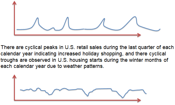
Seasonal effects are observed within a calendar year, e.g., spikes in sales over Christmas, while cyclical effects span time periods shorter or longer than one calendar year, e.g., spikes in sales due to low unemployment rates.<br>
One characteristic of seasonal patterns is their tendency of repeating themselves every year. In deterministic seasonality, there is an exact year-to-year repetition. In stochastic seasonality, the year-to-year repetition can be approximate. In business and economics, seasonality is pervasive.
Seasonality in a series can be examined by removing it, then modeling and forecasting the seasonally adjusted time series. One application of this strategy is an instance when non-seasonal fluctuations are the explicit forecast of interest, a common scenario in macroeconomics.
Regression on seasonal dummies is an important method of modeling seasonality. Assuming that there are \(s\) seasons in a year. Then the pure seasonal dummy model is:
$$ { y }_{ t }=\sum _{ i=1 }^{ s }{ { \gamma }_{ i }{ D }_{ it } } +{ \varepsilon }_{ t } $$
Where \({ D }_{ it }\) indicates whether we are in the \(i\)th quarter. The regression is on an intercept whereby in each season, a different intercept is permitted. The \(\gamma\)’s are referred to as the seasonal factors. Their role is to summarize the annual seasonal pattern. We will end up with similar \(\gamma\)’s, in the event that seasonality is absent. In that case, all the seasonal dummies can be dropped and an intercept included in the usual manner.
\(s – 1\) seasonal dummies and an intercept can be included rather than a full set of \(s\) seasonal dummies being included. The seasonal increment or decrement relative to the omitted season is determined by the coefficients on the seasonal dummies, while the omitted season’s intercept is given by the constant term.
We can also include a trend, and the model will change to:
$$ { y }_{ t }={ \beta }_{ 1 }{ TIME }_{ t }+\sum _{ i=1 }^{ s }{ { \gamma }_{ i }{ D }_{ it } } +{ \varepsilon }_{ t } $$
We can extend the concept of seasonality to accommodate more general calendar effects. One form of calendar effect is standard seasonality. Other forms are:
In holiday variation, the idea is that over time, there can be changes in some holidays’ dates. The best example is the Easter holiday whose date differs despite arriving at approximately the same time each year. The timing of such holidays partly affects the behavior of most series and such our forecasting models should track them. Dummy variables are used to handle holiday effects, an Easter Dummy is a good example.
In trading-day variations, the number of trading days or business days in a month is not the same. This consideration should, therefore, be taken into account when some series are modeled or forecasted.
The complete model that takes into account the likelihood or holiday or trading day variation is written as:
$$ { y }_{ t }={ \beta }_{ 1 }{ TIME }_{ t }+\sum _{ i=1 }^{ s }{ { \gamma }_{ i }{ D }_{ it } }+\sum _{ i=1 }^{ { V }_{ 1 } }{ { \delta }_{ i }^{ HD }{ HDV }_{ it }+ } \sum _{ i=1 }^{ { V }_{ 2 } }{ { \delta }_{ i }^{ TD }{ TDV }_{ it }+ } { \varepsilon }_{ t } $$
In the above equation, there are \({ V }_{ 1 }\) holiday variables denoted by \(HDV\), and \({ V }_{ 2 }\) trading-day variables denoted as \(TDV\). The ordinary least square can be a good estimation of this standard regression equation.
Let’s construct an \(h\)-step-ahead point forecast, \({ y }_{ T+h,T }\) at time \(T\).
The full model is:
$$ { y }_{ t }={ \beta }_{ 1 }{ TIME }_{ t }+\sum _{ i=1 }^{ s }{ { \gamma }_{ i }{ D }_{ it } } +\sum _{ i=1 }^{ { V }_{ 1 } }{ { \delta }_{ i }^{ HD }{ HDV }_{ it }+ } \sum _{ i=1 }^{ { V }_{ 2 } }{ { \delta }_{ i }^{ TD }{ TDV }_{ it }+ } { \varepsilon }_{ t } $$
At time \(T + h\):
$$ { y }_{ T+h }={ \beta }_{ 1 }{ TIME }_{ T+h }+\sum _{ i=1 }^{ s }{ { \gamma }_{ i }{ D }_{ i,T+h } } +\sum _{ i=1 }^{ { V }_{ 1 } }{ { \delta }_{ i }^{ HD }{ HDV }_{ i,T+h }+ } \sum _{ i=1 }^{ { V }_{ 2 } }{ { \delta }_{ i }^{ TD }{ TDV }_{ i,T+h }+ } { \varepsilon }_{ T+h } $$
The right side of the equation is projected on what is provided at time \(T\), to obtain the forecast.
$$ { y }_{ T+h,T }={ \beta }_{ 1 }{ TIME }_{ T+h }+\sum _{ i=1 }^{ s }{ { \gamma }_{ i }{ D }_{ i,T+h } } +\sum _{ i=1 }^{ { V }_{ 1 } }{ { \delta }_{ i }^{ HD }{ HDV }_{ i,T+h }+ } \sum _{ i=1 }^{ { V }_{ 2 } }{ { \delta }_{ i }^{ TD }{ TDV }_{ i,T+h } } $$
The unknown parameters are then replaced by the estimates, to ensure this point forecast is operational:
$$ { \hat { y } }_{ T+h,T }={ \hat { \beta } }_{ 1 }{ TIME }_{ T+h }+\sum _{ i=1 }^{ s }{ { \hat { \gamma } }_{ i }{ D }_{ i,T+h } } +\sum _{ i=1 }^{ { V }_{ 1 } }{ { \hat { \delta } }_{ i }^{ HD }{ HDV }_{ i,T+h }+ } \sum _{ i=1 }^{ { V }_{ 2 } }{ { \hat { \delta } }_{ i }^{ TD }{ TDV }_{ i,T+h } } $$
The next concern is how to form an interval forecast. The regression disturbance is assumed to be normally distributed. An interval forecast of 95% ignoring parameter estimation uncertainty is:
$$ { y }_{ T+h,T }\pm 1.96\sigma $$
We have to apply the following for internal forecast to be operational:
$$ { \hat { y } }_{ T+h,T }\pm 1.96\hat { \sigma } $$
The density forecast is another concept that will need to be formed. The assumption here is that trend regression disturbance is a normal distribution. The density forecast is written as follows, with parameter estimation uncertainty being ignored:
$$ N\left( { y }_{ T+h,T },{ \sigma }^{ 2 } \right) $$
The standard deviation of the disturbance in the trend regression is given as \(\sigma\). Therefore, the operational density forecast is given as:
$$ N\left( { \hat { y } }_{ T+h,T },{ \hat { \sigma } }^{ 2 } \right) $$
A mortgage analyst produced a model to predict housing starts (given in thousands) within California in the US. The time series model contains both a trend and a seasonal component and is given by the following:
$$ y_t = 0.2×Time_t+15.5 + 4.0 × D2t + 6.4× D3t + 0.5× D4t $$
The trend component is reflected in variable TIME(t), where (t) month and seasons are defined as follows:
| Season | Months | Dummy |
| Winter | December, January, and February | – |
| Spring | March, April, and May | D(2t) |
| Summer | June, July, and August | D(3t) |
| Fall | September, October, and November | D(4t) |
The model starts in April 2019; for example, y(T+1) refers to May 2019.
What does the model predict for March 2020?
The correct answer is A.
The model is given as:
$$ y_t = 0.2×Time_t+15.5 + 4.0 × D2t + 6.4×D3t + 0.5×D4t $$
Important: Since we have three dummies and an intercept, quarterly seasonality is reflected by the intercept (15.5) plus the three seasonal dummy variables (D2, D3, and D4).
If y(T+1) = May 2019, then March 2020 = y(T + 11)
Finally, note that March falls under D(2t)
$$ y(T+11) = 0.20 × 11 + 15.5 + 4.0 × 1 = 21.7 $$
Thus, the model predicts 21,700 housing starts in March 2020.
Offered by AnalystPrep


