


Classifications and Key Concepts of Cr ...
Classification Default Model and Value-based Valuations A borrower’s default constitutes default risk. On... Read More

After completing this reading, you should be able to:
Banks’ internal classification methods are somewhat different from agencies’ ratings assignment processes. Nevertheless, sometimes their underlying processes are analogous; when banks adopt judgmental approaches to credit quality assessment, the data considered and the analytical processes are similar.
An expert-based approach relying on judgment will require significant experience and repetitions in order for many judgments to converge. In other words, judgment-based schemes need long-lasting experience and repetitions, under a constant and consolidated method, to assure the convergence of judgments. As we would expect, therefore, internal rating systems take time to develop. The failure to attain consistency under the expert-based approach can be attributed to several factors, some of which are outlined below:
However, there is no proven inferiority or superiority of expert-based approaches versus formal ones, based on quantitative analysis such as statistical models.
Earlier on, we looked at the qualities of a good rating system – objectivity and homogeneity, specificity, measurability, and verifiability. We can compare agencies’ ratings and internal expert-based rating systems along similar lines:
$$ \begin{array}{l|cc} \textbf{Quality} & \textbf{Compliance level} & {} \\ \hline \text{} & \text{Agencies’} & \text{Internal experts-} \\ {} & \text{ratings} & \text{based ratings} \\ \hline \text{Objectivity and Homogeneity} & {73\%} & {30\%} \\ \hline \text{Specificity} & {100\%} & {75\%} \\ \hline \text{Measurability and Verifiability} & {75\%} & {25\%} \\ \end{array} $$
A scoring model is a model in which various variables are weighted in varying ways and result in a score. This score subsequently forms the basis for a decision. In finance, scoring models combine quantitative and qualitative empirical data to determine the appropriate parameters for predicting default. Linear discriminant analysis (LDA) is a popular statistical method of developing scoring models.
The linear discriminant analysis classifies objects into one or more groups based on a set of descriptive features. Models based on LDA are reduced-form models due to their dependency on exogenous variable selection, default composition, and the default definition. The variables used in an LDA model are chosen based on their estimated contribution (i.e., weight) to the likelihood of default. These variables are both qualitative and quantitative. Examples are the skill and experience of management and the liquidity ratio, respectively. The contributions of each variable are added to form an overall score, called Altman’s
Altman Z-score is essentially a bankruptcy prediction tool published by Edward I. Altman in 1968. Mr. Altman worked with 5 ratios: net working capital to total assets ratio, earnings before interest and taxes to total assets ratio, retained earnings to total assets ratio, market value of equity to total liabilities ratio, and finally, sales to assets ratio. Below is the LDA model proposed by Altman:
$$ \begin{align*} \text{Z}=1.21 \text{x}_{ 1 }+1.4 \text{x}_{ 2 }+3.3 \text{x}_{ 3 }+0.6 \text{x}_{ 4 }+0.999 \text{x}_{ 5 } \end{align*}$$
where:
\(\text{x}_{ 1 }=\text{Working capital}/\text{total assets}\).
\(\text{x}_{ 2 }=\text{Retained earnings}/\text{total assets}\).
\(\text{x}_{ 3 }=\text{EBIT}/\text{total assets}\).
\(\text{x}_{ 4 }=\text{Equity market value}/\text{face value of term debt}\).
\(\text{x}_{ 5 }=\text{Sales}/\text{total assets}\).
In this model, the higher the Z-score, the more likely it is that a firm will be classified in the group of solvent firms. Altman worked with a Z-score range from -5.0 to +20.0, although higher scores may occur if a company has a high equity value and/or low level of liabilities.
A Z-score cutoff, also known as the discriminant threshold, is used to categorize firms into two groups: solvent firms and insolvent firms. Altman set the Z-score cutoff at Z = 2.675. Firms with a score below 2.675 are categorized as insolvent while those with a score above 2.675 are categorized as solvent.
A borrower’s credit rating reflects their probability of default. The higher the rating, the more financially reliable a borrower is considered to be. This implies that higher-rated issues have a lower probability of default. In fact, the highest-rated issues almost never default even over a significant period of, say, 10 years. The lowest-rated issues, on the other hand, often default early and are almost assured of default after a 10-year period.
A rating migration matrix gives the probability of a firm ending up in a certain rating category at some point in the future, given a specific starting point. The matrix, which is basically a table, uses historical data to show exactly how bonds that begin, say, a 5-year period with an Aa rating, change their rating status from one year to the next. Most matrices show one-year transition probabilities.
Transition matrices demonstrate that the higher the credit rating, the lower the probability of default.
The table below presents an example of a rating transition matrix according to S&P’s rating categories:
$$ \textbf{One-year transition matrix}$$
$$ \small{\begin{array}{l|c|c|c|c|c|c|c|c} \textbf{Initial}& {} && && & {} & {} & {} \\ \textbf{Rating} & \textbf{AAA} & \textbf{AA} & \textbf{A} & \textbf{BBB} & \textbf{BB} & \textbf{B} & \textbf{CCC} & \textbf{Default}\\ \hline \text{AAA} & {90.81\%} & {8.33\%} & {0.68\%} & {0.06\%} & {0.12\%} & {0.00\%} & {0.00\%} & {0.00\%} \\ \text{AA} & {0.70\%} & {90.65\%} & {7.79\%} & {0.64\%} & {0.06\%} & {0.14\%} & {0.02\%} & {0.00\%} \\ \text{A} & {0.09\%} & {2.27\%} & {91.05\%} & {5.52\%} & {0.74\%} & {0.26\%} & {0.01\%} & {0.06\%} \\ \text{BBB} & {0.02\%} & {0.33\%} & {5.95\%} & {86.93\%} & {5.30\%} & {1.17\%} & {0.12\%} & {0.18\%} \\ \text{BB} & {0.03\%} & {0.14\%} & {0.67\%} & {7.73\%} & {80.53\%} & {8.84\%} & {1.00\%} & {1.06\%} \\ \text{B} & {0.00\%} & {0.11\%} & {0.24\%} & {0.43\%} & {6.48\%} & {83.46\%} & {4.07\%} & {5.20\%} \\ \text{CCC} & {0.22\%} & {0.00\%} & {0.22\%} & {1.30\%} & {2.38\%} & {11.24\%} & {64.86\%} & {19.79\%} \\ \end{array}}$$
This measures the likelihood of default over a single time period of length k. It is simply the fraction of the cohort that survives to the end of the period:
$$ \begin{align*} \text{ PD }_\text{ k }=\frac { \text{defaulted}_\text{ k }^\text{ t+k } }{ \text{cohort}_\text{ t } } \end{align*}$$
Where:
\(\text{ PD }_{\text{ k }}\)= Probability of default.
\(\text{defaulted}_\text{ k }^\text{ t+k }\)= Number of issuer names (members of the cohort) that have defaulted between time \(\text{t}\) and time \(\text{t+k}\).
The K-horizon cumulative default rate is defined as the probability of default from the time of cohort formation up to and including time horizon K $$ \begin{align*} \text{ PD }_\text{ k }^\text{ cumulative }=\frac { \sum _{ \text i=\text t }^{\text i=\text{t}+\text{k} }{ \text{ defaulted }_\text{ i } } }{\text{ cohort}_\text{ t } } \end{align*}$$. If K is 5 years, for example, the cumulative probability of default in year 5 means the probability of an issuer name defaulting in either year 1, 2, 3, 4 or 5 (i.e., the sum of defaults in years 1, 2, 3, 4, and 5).
The following table gives the cumulative default rates provided by Moody’s.
$$ \textbf{Cumulative Ave Default Rates (%) (1970-2009, Moody’s)} $$
$$ \begin{array}{c|c|c|c|c|c|c|c} \textbf{ } & \textbf{1} & \textbf{2} & \textbf{3} & \textbf{4} & \textbf{5} & \textbf{7} & \textbf{10} \\ \hline \text{ Aaa} & {0.000} & {0.012} & {0.012} & {0.037} & {0.105} & {0.245} & {0.497} \\ \hline \text{ Aa} & {0.022} & {0.059} & {0.091} & {0.159} & {0.234} & {0.348} & {0.542} \\ \hline \text{A } & {0.051} & {0.165} & {0.341} & {0.520} & {0.717} & {1.179} & {2.046} \\ \hline \text{ Baa} & {0.176} & {0.494} & {0.912} & {1.404} & {1.926} & {2.996} & {4.551}\\ \hline \text{ Ba} & {1.166} & {3.186} & {5.583} & {8.123} & {10.397} & {14.318} & {19.964} \\ \hline \text{ B} & {4.546} & {10.426} & {16.188} & {21.256} & {25.895} & {34.473} & {44.377} \\ \hline \text{ Caa-C} & {17.723} & {29.384} & {38.682} & {46.094} & {52.286} & {59.771} & {71.376} \\ \end{array} $$
According to the table, an issuer name with an initial credit rating of Ba has a probability of 1.166% of defaulting by the end of the first year, 3.186% by the end of the second year, and so on. We can interpret the other default rates in a similar manner.
The marginal default rate is the probability that an issuer name that has survived in a cohort up to the beginning of a particular interval k will default by the end of the time interval.
$$ \begin{align*} \text{ PD }_\text{ k }^\text{ marginal }=\text{ PD }_\text{ t+k }^\text{ cumulative }-\text{ PD }_\text{ k }^\text{ cumulative } \end{align*}$$
For discrete intervals, the annualized default rate can be computed as follows:
$$ \begin{align*} \text{ ADR }_\text{ t }=1-\sqrt [ \text{t} ]{ \left( 1-\text{ PD }_\text{ t }^\text{ cumulative } \right) } \end{align*}$$
For continuous intervals,
$$ \begin{align*} \text{ ADR }_\text{ t }=-\frac { \text{ln}\left( 1-\text{ PD }_\text{ t }^\text{ cumulative } \right) }{ \text{t} } \end{align*}$$
The hazard rate (also called default intensity) is the probability of default for a certain time period conditional on no earlier default. It is the parameter driving default. It is usually represented by the parameter \(\lambda\). The probability of default over the next small time interval, dt, is \({ \lambda }\text {dt}\).
$$ \text{PD} \left( \text t,\text t+{\text {dt}} \right)={ \lambda } \text{dt} $$
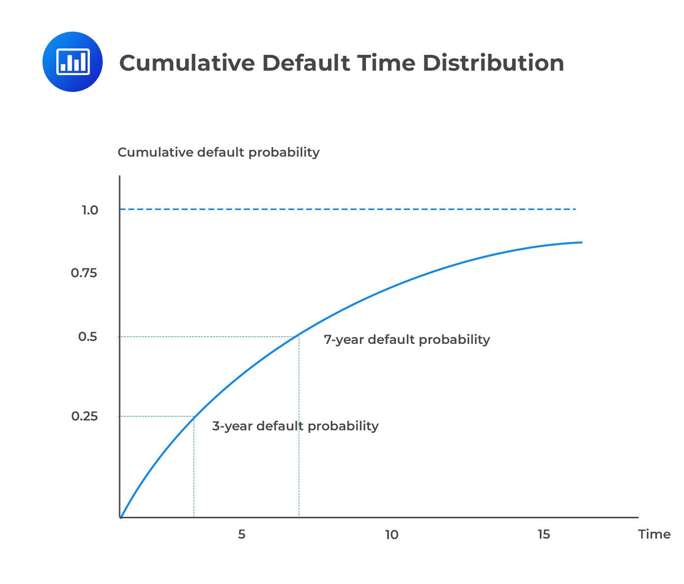
Using \({\text t }^{ * }\) to represent the time of default, the cumulative default time distribution F(t) gives the probability of default over (0,t).
$$ \text P\left[ { \text t }^{ * }< {\text t} \right] \equiv {\text F}(\text t)=1-{ \text e }^{ -\lambda {\text t} } $$
The survival distribution is as follows:
$$ {\text P}\left[ { \text t }^{ * }\ge {\text t} \right] =1-{\text P}\left[ {\text t }^{ * }<\quad {\text t} \right] =1-{\text F}\left( \text t \right) { =\text e }^{ -\lambda {\text t} } $$
Note that the default time distribution and the survival distribution add up to 1 at each point in time.
As t grows very large, the survival probability converges at 0 while the default probability converges at 1. The intuition is that the probability of default increases as we peer deeper into the future. Even the best-rated bond, say AAA, will eventually default.
 $$ \textbf{Default Time Density Function} $$
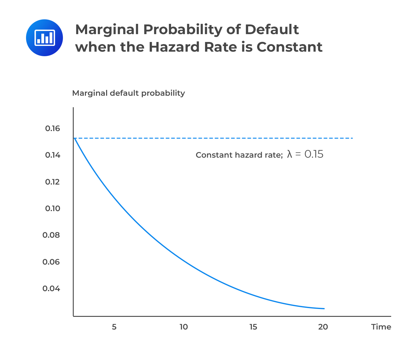
The default time density function is the derivative of the default time distribution, w.r.t t. Sometimes, it is called the marginal default probability.
$$ \cfrac { \partial }{ \partial {\text t} } {\text P}\left[ {\text t }^{ * }< {\text t} \right] ={ \text F }^{ \prime \left(\text t \right) }=\lambda { \text e }^{ -\lambda {\text t} }$$
The default time density function is always positive because default risk tends to “accumulate” over time. However, the rate of increase depends on \({\lambda}\). With a big value, default risk will increase at a quick pace.
The survival probability, again, decreases over time.
$$ \cfrac { \partial }{ \partial {\text t} } {\text P}\left[ { \text t }^{ * }\ge {\text t} \right] ={ -\text F }^{ \prime \left( \text t \right) } =-\lambda { \text e }^{ -\lambda {\text t} } $$
If we hold the hazard rate at a constant value \({\lambda}\), we will find that the marginal default probability is positive but declining. The implication is that although the probability of default increases the further out we peer into the future, the rate at which this probability accumulates declines.
 Conditional Default Probability
The conditional default probability gives the probability of default over some horizon \((\text t,\text t+\tau)\) given that there has been no default prior to time t.
$$ \text P\left( { \text t }^{ * } < {\text t}+\tau |{ \text t }^{ * } > {\text t} \right) =\cfrac { \text p\left[ {\text t }^{ * } > \text t\cap { \text t }^{ * } < {\text t}+\tau \right] }{ \text p \left[ { \text t }^{ * } > {\text t} \right] } \ $$
For example, the conditional one-year probability of default, assuming survival during the first year, is equal to the difference between the unconditional two-year PD and the unconditional one-year PD divided by the one-year survival probability.
The conditional one-year PD is given by:
$$ \cfrac { \text{Unconditional two year PD}-\text{Unconditional one year PD} }{ \text{One year survival PD} } $$
Compute the one-, two-, and three-year cumulative default probabilities and conditional default probabilities, assuming that the hazard rate is 0.10
$$ \begin{array}{c|c|c|c|c} \bf{\text t} & {\textbf{Cumulative PD} \\ {\left[ 1-{ \text{e} }^{ -\lambda \text{t} } \right] } } & {\textbf{Survival Prob.} \\ {\left[{ \text{e} }^{ -\lambda \text{t} } \right] } } & \textbf{PD(t,t+1))} & {\textbf{Conditional PD} \\ \textbf{given survival until} \\ \textbf{time t} } \\ \hline 1 & {1-{ \text{e} }^{ -0.1\times 1 } \\ {=9.52\%} } & {{ \text{e} }^{ -0.1\times 1 } \\ {=90.48\%} } & {9.52\%} & {-} \\ \hline 2 & {1-{ \text{e} }^{ -0.1\times 2 } \\ {=18.13\%} } & {{ \text{e} }^{ -0.1\times 2} \\ {=81.87\%} } & { \left( 18.13\%-9.52\% \right) \\ {=8.61\%} } & { {\frac {8.61\%}{90.48\%} } \\ {=9.52\%} } \\ \hline 3 & {1-{ \text{e} }^{ -0.1\times 3 } \\ {=25.92\%} } & {{ \text{e} }^{ -0.1\times 3} \\ {=74.08\%} } & { \left( 25.92\%-18.13\% \right) \\ {=7.79\%} } & { {\frac {7.79\%}{81.87\%}} \\ {=9.52\%} } \end{array} $$
Notice that the two conditional probabilities are equal.
Default probabilities can also be extracted from market prices. The resulting probabilities are risk-neutral. This implies that the probabilities include compensation for both the loss given default and bearing the risk of default and uncertainties that come along with it.
The spread over the risk-free rate on a bond that is defaultable with maturity T is denoted by \(\text z_{\text t}\), and the constant risk-neutral hazard rate at time T is \(\lambda_{\text T}^{*}\).
If recovery is zero,
$$ { \lambda }_{ \text T }^{ * }={ \text z }_{ \text t } $$
The equation above implies that the hazard rate is equal to the spread.
For small values of x, we can use the approximation \(\text e^{\text x}=1+ \text x\) so that:
$$ { \text z }_{\text t }=1-{\text e }^{ -{ \lambda }_{\text T }^{ * } } $$
After a bit of algebraic manipulation, it can be shown that the average default intensity over the life of the bond is approximately,
$$ \cfrac { \text S }{ 1-{\text R} } $$
where s is the spread of the bond’s yield over the risk-free rate, and R is the recovery rate.
Example: With a five-year bond that has a spread of 200 bps and a recovery rate of 40%, for example, the average default intensity (hazard rate) = 0.02/0.6 = 0.0333.
Recovery rates are a key metric in the assessment of credit risk, representing the proportion of principal and accrued interest that can be recuperated in the event of a borrower’s default. It is often expressed as a percentage of face value that creditors recover after a firm’s default.
Historical data show variations in average recovery rates among different bond classes. For example:
During financial distress, as more firms default, more assets enter the market, pushing down their sale prices. Consequently, this affects recovery rates negatively:
The dependency of recovery rates on default rates has significant implications for lenders and investors. A high default rate can not only mean more frequent losses but also lower recoveries on investment, leading to a compounded negative effect on returns.
Studies have noted this negative relationship, pointing out that recovery rates on corporate bonds tend to drop in years when the default rate is high, and vice versa. The correlation indicates that default and recovery rates are inversely related, a factor which must be considered when estimating potential losses from credit risks.
A credit default swap (CDS) is a financial derivative instrument that works similarly to insurance on credit events. It is primarily used to manage and trade credit risks associated with various financial instruments, typically bonds. They grew rapidly in popularity until 2007 due to their ability to ‘insure’ against the default of a particular company—known as the reference entity. Following a default event, CDS contracts facilitate a transfer of credit risk from one party to another.
Before looking at how we can go about deriving a hazard rate curve from CDS spread, let’s remind ourselves of a few things about credit default swaps.
However, when CDS trade points upfront, a percent of the principal is paid by the protection buyer. This impacts the counterparty credit risk of the contract rather than its pricing. In addition, some collateral has to be provided at the onset.
Quarterly spread payments (called the free leg) have to be made by the protection buyer until the maturity date of the contract, unless and until the reference entity undergoes an event of default.
The protection seller makes a payment, called the contingent leg, only if there is a default. This payment leg is equal to the loss given default.
At the onset, the expected present value of the free leg is equal to that of the contingent leg.
Assume that we wish to find the default curve for a company. Let’s further assume that we have only a single CDS spread, for a term of five years. As such, we will have a single hazard estimate. The protection buyer will pay the spread in quarterly installments. These will be dates t = 0.25, 0.5,…1.5, 5. The installments will be a function of the unknown hazard rate λ, which is linked to the probability of survival up to time t, \({ \pi }_{ \text t }\), as follows:
$$ { \pi }_{\text t }=1-{\text e }^{ -\lambda {\text t} } $$
We will need to work with the CDS valuation equation which equates the PV of the free leg to the PV of the contingent leg.
The PV of the free leg is given by:
$$ \cfrac { { \text S }_{ \tau } }{ 4\times { 10 }^{ 4 } } \sum _{ \text u=1 }^{ { 4 }{ \tau } }{ { {\text p }_{ 0.25{\text u} } } } \left[ { \text e }^{ -\lambda \left( \cfrac { \text u }{ 4 } \right) }+0.5\left( { \text e }^{ -\lambda \cfrac { \left( \text u-1 \right) }{ 4 } }-{ \text e }^{ -\lambda \left( \cfrac { \text u }{ 4 } \right) } \right) \right] $$
While the PV of the contingent leg is given by:
$$ \left( 1-\text R \right) \sum _{\text u=1 }^{ { 4 }{ \tau } }{ { { \text p }_{ 0.25{\text u} } } } \left( {\text e }^{ -\lambda \cfrac { \left( \text u-1 \right) }{ 4 } }-{\text e }^{ -\lambda \left( \cfrac { \text u }{ 4 } \right) } \right) $$
where:
Provided all the variables are known, we can substitute them in the equation and get the value of λ
$$ \begin{array}{c|c} \textbf{Reference entity} & \textbf{Merrill Lynch} \\ \hline \text{Initiation Date} & \text{October 1 2008} \\ \hline {\text{Single five-year CDS spread}, \text s_\tau} & \text{445 bps} \\ \hline \text{Hazard Rate} & \text{Constant} \\ \hline \text{Recovery Rate, R} & {40\%} \\ \hline \text{Swap curve} & \text{Flat} \\ \hline \text{Continuously compounded spot rate} & {4.5\%} \\ \hline {\text{Term of the CDS}, \tau} & \text{5 years} \\ \end{array} $$
We can work out a value for \(\lambda\) as follows:
$$ \cfrac { 445 }{ 4\times { 10 }^{ 4 } } \sum _{\text u=1 }^{ { 4 }_{ \tau } }{ {\text e }^{ 0.045\left( \frac { \text u }{ 4 } \right) } } \left[ { \text e }^{ -\lambda \left( \frac { \text u }{ 4 } \right) }+0.5\left( { \text e }^{ -\lambda \frac { \left(\text u-1 \right) }{ 4 } }-{ \text e }^{ -\lambda \left( \frac { \text u }{ 4 } \right) } \right) \right] $$
$$ =\left( 1-0.4 \right) \sum _{ \text u=1 }^{ { 4 }{ \tau } }{ {\text e }^{ 0.045\left( \frac { \text u }{ 4 } \right) } } \left( {\text e }^{ -\lambda \frac { \left( \text u-1 \right) }{ 4 } }-{\text e }^{ -\lambda \left( \frac {\text u }{ 4 } \right) } \right) $$
Solving this gives \(\lambda\)=0.0741688
The CDS-bond basis is defined as the difference between the CDS spread and the bond yield spread for a specific company.
$$ \text{CDS-Bond Basis} = \text{CDS Spread} – \text{Bond Yield Spread}$$
Under ideal conditions, the basis should be near zero. This is based on arbitrage arguments, which suggest that the cost of credit protection acquired through a CDS should, in theory, align with the extra yield demanded by the market for holding a risky bond over a risk-free bond.
In practice, the CDS-bond basis can deviate from zero due to various reasons:
The historical performance of the CDS-bond basis has varied:
Default probabilities calculated from historical data represent “real-world” or physical probabilities of default. These probabilities are inferred from past occurrences of defaults within certain classifications or ratings assigned to companies. Credit rating agencies like Standard & Poor’s publish average cumulative default probabilities based on extensive historical data. For example, they may calculate the seven-year average cumulative default probability by analyzing the historical performance of companies within each credit rating category.
On the other hand, default probabilities calculated from credit spreads are referred to as “risk-neutral” probabilities. Credit spreads are the risk premiums over the “risk-free” rate that investors demand for taking on the credit risk of a corporate bond, reflecting the market’s perception of credit risk. These spreads can be used to calculate an implied hazard rate, which can then be translated into a risk-neutral default probability.
Hazard rates implied by credit spreads tend to be higher than those calculated from historical default rates. This suggests that the market demands a premium for bearing credit risk, which goes beyond an actuarial estimate of the cost of defaults.
Moreover, this risk premium or excess return increases as the credit quality declines, indicating that investors are typically compensated more generously for assuming higher credit risks. The discrepancy between the two estimates becomes more pronounced during periods of financial stress, such as the Global Financial Crisis when credit spreads soared significantly.
The choice between using real-world and risk-neutral default probabilities depends on the application. For valuation purposes, risk-neutral default probabilities, derived from credit spreads, are typically used, consistent with the principle of using market-based valuations. For scenario analysis, where the goal is to assess different potential future states, it is more appropriate to use real-world probabilities that consider historical default rates.
Real-world, or physical, default probabilities are derived from historical data. These are probabilities published by rating agencies, based on historical default rates of entities within various credit rating categories. They provide an empirical measure of the frequency of default observed in the past and are seen as an estimate of the actual likelihood that a company will default on its debt obligations in the future.
Risk-neutral default probabilities, in contrast to real-world probabilities, are derived from financial markets, particularly from credit spreads. These are higher than real-world default probabilities because they include not only the actual historical likelihood of default but also market participants’ risk aversions and the premium that investors demand for bearing credit risk. Essentially, these probabilities are a measure of the market’s current expectations regarding the risk of default.
Risk-neutral default probabilities are greater than real-world default probabilities because they reflect the market’s demand for risk premiums on top of the historical likelihood of default. The difference accounts for the extra compensation investors need to hold risky debt over risk-free assets.
The distinction between the two comes down to the expected asset growth rate:
For Valuation: Risk managers and financial analysts should use risk-neutral probabilities when valuing financial instruments, such as bonds or derivatives. This conforms to the underlying principle of risk-neutral valuation, where all risk premiums are reflected in discounted future cash flows.
For Scenario Analysis: Real-world probabilities are more appropriate for assessing various potential future outcomes. They incorporate actual historical experience and provide a basis for estimating frequencies of future default under different economic scenarios.
The Merton model is used to assess a company’s credit risk by modeling the company’s equity as a call option on its assets. It is built upon the Black-Scholes pricing model and seeks to establish a link between default and a firm’s capital structure.
In its simplest form, the Merton model makes a set of assumptions:
These assumptions have certain implications. If the markets are perfect, for example, then the value of the firm equals the value of debt plus the value of equity.
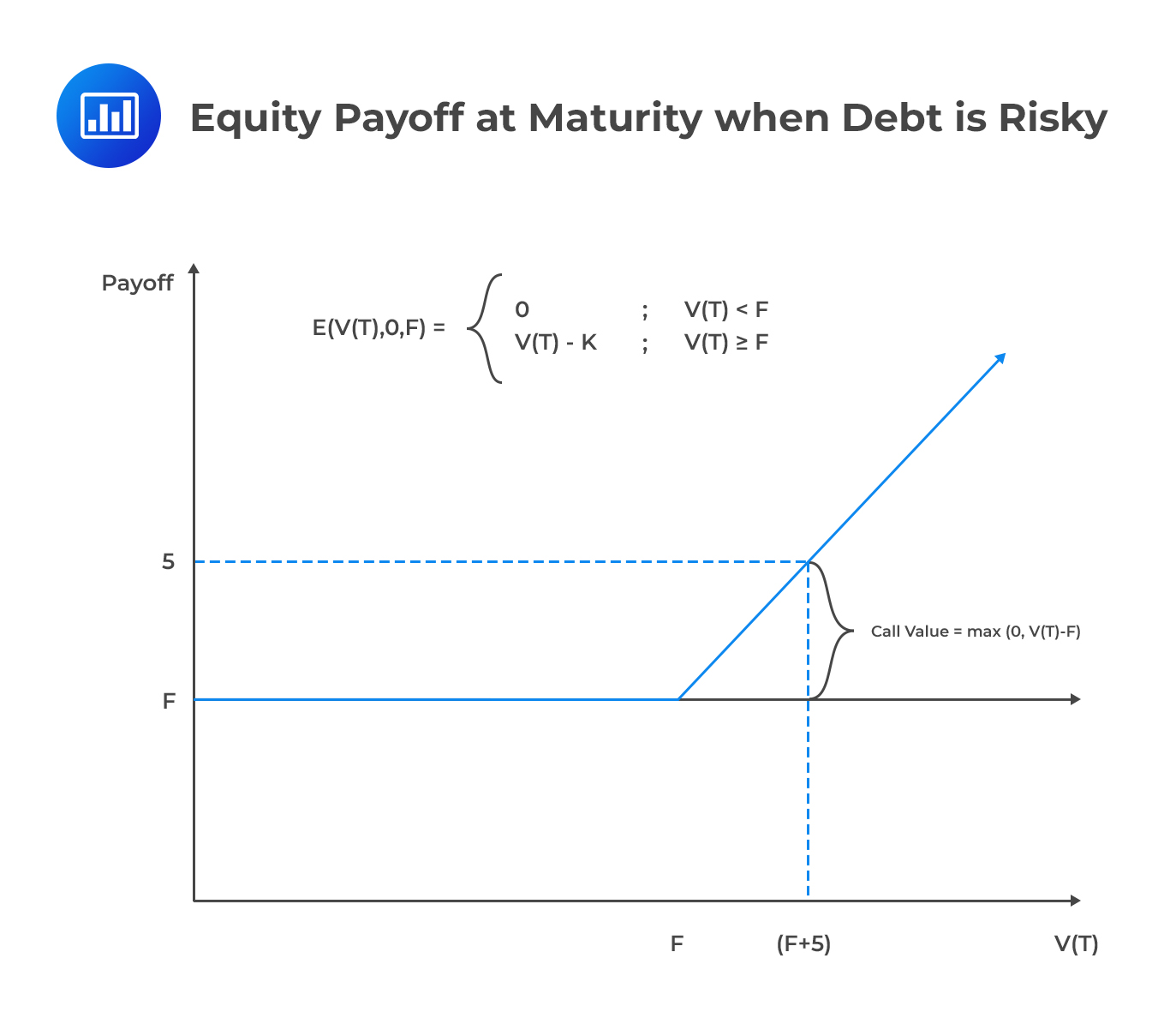
In line with these assumptions, let’s assume that a firm has a single outstanding zero-coupon debt with a face value (principal amount) F, payable at time T. Now, there are two possible scenarios. First, the value of the firm at time T, \({\text{V}}_{\text{T}}\) could be large enough to pay the principal amount, in which case, shareholders have a claim over the balance, i.e., \({\text{V}}_{\text{T}}\)-F. Secondly, the value of the firm at time T could be insufficient such that the firm is unable to settle the principal amount, in which case, equity holders receive nothing.
Looking closely, the two possible scenarios and their payoffs pretty much resemble a call option, with the underlying instrument as firm value and the principal amount as the exercise price. The value of equity at time T can therefore be represented as:
$$ { \text{E} }_{ \text{T} }=\text{Max}\left( { \text{V} }_{ \text{T} }-\text{F},0 \right) $$
A simplified example will help further drive the concept home.
Assume that a firm has issued zero-coupon debt that requires it to pay $160m to debt holders at maturity. Further, assume that the firm has no other creditors. If the total value of the firm at maturity is $180m, what’s the firm’s value of equity? What is the value of equity given a firm value of $140m at maturity?
$$ { \text{E} }_{ \text{T} }=\text{Max}\left( { \text{V} }_{ \text{T} }-\text{F},0 \right) $$
In the first case,
$$ { \text{E} }_{ \text{T} }=\text{Max}\left( 180-160,0 \right) =20 $$
In the second case,
$$ { \text{E} }_{ \text{T} }=\text{Max}\left( 140-160,0 \right) =0 $$
The following figure illustrates the fact that the payoff for equity is equal to the payoff for a long call option.
 Calculating the Value of Debt
How about the payoff for debt? If we assume that a debt is risk-free and payment of the principal amount F is guaranteed, the payoff would be F, regardless of firm value at maturity. In the presence of risk, however, the debt holder receives an amount lower than the anticipated payment if the firm value, \({\text{V}}_{\text{T}}\) is less than F. In other words, we are saying that if \({\text{V}}_{\text{T}} < \text F\) at maturity, then the amount received by the debt holder will be reduced by \(\text F-\text V_{\text T}\).
The payoff for debt is pretty much like that of a combination of a long position in a T-bill with a face value of F and a short position on the firm value with an exercise price of F. In other words, holders of risky debt effectively buy risk-free debt and write a put option on the value of the firm with an exercise price equal to the face value of the debt. We can therefore represent the value of debt, \({\text{D}}_{\text{T}}\), as follows:
$$ { \text{D} }_{ \text{T} }=\text{F}-\text{max}\left( \text{F}-\text{V}_{ \text{T} },0 \right) $$
Assume that a firm has issued zero-coupon debt that requires it to pay $160 million to debt holders at maturity. In addition, assume that the firm has no other creditors. If the total value of the firm at maturity is $180m, what’s the firm’s value of debt? What is the value of debt given a firm value of $140m at maturity?
$$ { \text{D} }_{ \text{T} }=\text{F}-\text{max}\left( \text{F}-\text{V}_{ \text{T} },0 \right) $$
In the first case,
$$ { \text{D} }_{ \text{T} }=160-\text{max}\left( 160-180,0 \right) =160 $$
In the second case,
$$ { \text{D} }_{ \text{T} }=160-\text{max}\left( 160-140,0 \right) =140 $$
Note: It would also be correct to look at the payoff for debt as the value of a firm minus the payoff of a call option with exercise price equal to the principal amount of the debt.
To price the equity and the debt using the Black-Scholes formula for the pricing of a European call, we need to make additional assumptions:
Using E(V, F, T, t) to represent the value of equity,
$$ \text{E}\left(\text {V,F,T,t}\right) =\text{V}\times \text{N}\left( \text{d} \right) -{ \text{Fe} }^{ { -\text{r} }^{ \left( \text{T-t} \right) } }\times \text{N}\left( \text{d}-\sigma \sqrt { \text{T-t} } \right) $$
Where:
$$ \text{d}=\cfrac { \text{ln}\left( \cfrac { \text{V} }{ { { \text{Fe} } }^{ { -{ \text{r} } }^{ \left( { \text{T-t} } \right) } } } \right) }{ \sigma \sqrt { \text{T-t} } } +\cfrac { 1 }{ 2 } \sigma \sqrt { \text{T-t} } $$
V = Value of the firm.
F = Face value of the firm’s zero-coupon debt maturing at T (only liability).
\(\sigma\) = Volatility of the value of the firm.
r = Annual interest rate.
N = Cumulative normal distribution.
A firm has a current value of $100 million. Its only outstanding debt is a 3-year zero-coupon bond with a face value of $80 million. Compute the value of the firm’s equity at time=t given the following information:
$$ \begin{align*} \text{E}\left(\text {V,F,T,t}\right) & =\text{V}\times \text{N}\left( \text{d} \right) -{ \text{Fe} }^{ { -\text{r} }^{ \left( \text{T-t} \right) } }\times \text{N}\left( \text{d}-\sigma \sqrt { \text{T-t} } \right) \\ & =100\times \text{N}\left( \text{d} \right) -80{ \text{e} }^{ -0.05\times 3 }\times \text{N}\left( \text{d}-0.1\sqrt { 3 } \right) \\ \text{d} & =\cfrac { \text{ln}\left( \cfrac { \text{V} }{ { { \text{Fe} } }^{ { -{ \text{r} } }^{ \left( { \text{T-t} } \right) } } } \right) }{ \sigma \sqrt { \text{T-t} } } +\cfrac { 1 }{ 2 } \sigma \sqrt { \text{T-t} } \\ & =\cfrac { \text{ln}\left( \cfrac { 100 }{ 80{ { \text{e} } }^{ -0.05\times 3 } } \right) }{ 0.1\sqrt { 3 } } +\cfrac { 1 }{ 2 } 0.1\sqrt { 3 } =2.15435+0.086603=2.2410 \\ \text{E}\left(\text {V,F,T,t}\right) & = 100\times \text{N}\left(2.2410 \right)-68.85664 \times \text{N} \left(2.0678 \right) \end{align*} $$
From probability tables, \(\text{N}(2.241) = 0.9875 \text{ and } \text{N}(2.0678) = 0.9807\)
$$ \text{E}(\text{V,F,T,t})=98.75-67.52767=31.2223 $$
The value of equity is $31.2223 million
Note: The formula can also be computed as follows:
$$ { \text{E} }\left( { \text{V,F,T,t} } \right) =\text{V}\times \text{N}\left( { \text{d} }_{ 1 } \right) -{ { \text{Fe} } }^{ { -{ \text{r} } }^{ \left( { \text{T-t} } \right) } }\text{N}\left( { \text{d} }_{ 2 } \right) $$
Where:
$$ \begin{align*} { \text{d} }_{ 1 } & =\cfrac { \text{ln}\cfrac { \text{V} }{ \text{F} } +\left( \text{r}+\cfrac { { \sigma }^{ 2 } }{ 2 } \right) \left( \text{T-t} \right) }{ \sigma \sqrt { \text{T-t} } } \\ { \text{d} }_{ 2 } & ={ \text{d} }_{ 1 }-\sigma \sqrt { \text{T-t} } \end{align*} $$
and everything else defined as before.
There are two ways to compute the value of debt. First, we can use the fact that the payoff of risky debt equals the payoff of risk-free debt less the payoff of a put option on the firm with the face value of the debt as the exercise price. Using D(V,F,T,t) to represent the value of debt and p(V,F,T,t) to represent the price of the put option at time t,
$$ { \text{D} }\left( { \text{V,F,T,t} } \right) =\text{P}\left( \text{T} \right) \text{F}-{ \text{p} }\left( { \text{V,F,T,t} } \right) $$
Where \(\text{P}\left(\text{T}\right)\) is the price of a discount bond that matures at T.
A firm has a current value of $100 million. Its only outstanding debt is a 3-year zero-coupon bond with a face value of $80 million. Compute the value of the firm’s debt at t as a portfolio of risk-free debt and a short position in a put-on firm value with an exercise price of the face value of debt. You have been given the following information:
We have already established the value of equity as $31.2223 million.
$$ \begin{align*} { \text{D} }\left( { \text{V,F,T,t} } \right) & = { \text{Fe} }^{ { -\text{r} }^{ \left( \text{T-t} \right) } } -{ \text{p} }\left( { \text{V,F,T,t} } \right) \\ & = 80{ \text{e} }^{ -0.05\times 3 }-{ \text{p} }\left( { \text{V,F,T,t} } \right) \\ & = 80 \times 0.8607-{ \text{p} }\left( { \text{V,F,T,t} } \right) \\ & =68.86-{ \text{p} }\left( { \text{V,F,T,t} } \right) \end{align*} $$
Using put-call parity, we can determine the value of the put:
$$ \begin{align*} { \text{p} }\left( { \text{V,F,T,t} } \right) & = {\text{c}}_{\text{t}} + { \text{Fe} }^{ { -\text{r} }^{ \left( \text{T-t} \right) } } -V \\ & = 31.2223+80{ \text{e} }^{ -0.05\times 3 }-100 \\ & = 0.078938 \\ { \text{D} }\left( { \text{V,F,T,t} } \right) & = 68.86-0.078938=$68.78 \\ \end{align*} $$
The second method that can be used to determine the value of debt is by simply subtracting the value of equity from the value of the firm. In the example above, the value of the firm is $100m, while the value of equity is $31.2223m. The difference gives us the value of debt ($68.78m).
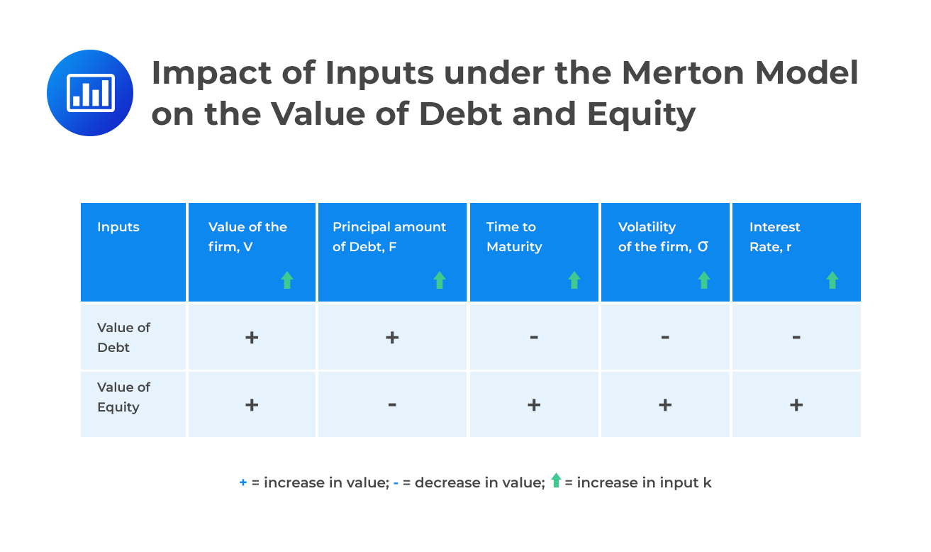
For a given value of the firm, the value of the debt is a decreasing function of the value of equity, which is the value of a call option on the value of the firm. Holding everything else equal, therefore, the table below summarizes how the value of debt and the value of equity are affected by various inputs under the Merton model:
The distance to default measures how far a firm’s asset value must fall, in terms of standard deviations, before default is triggered. It represents the number of standard deviations the firm’s asset value is away from the default point (typically the face value of debt).
A common definition of distance to default is the variable \( d_2 \) in the Black-Scholes-Merton framework, which can also be calculated as:
$$ DD = d_2 = \frac{\ln\left(\frac{V_0}{D}\right) + \left(r – \frac{1}{2} \sigma_V^2\right)T}{\sigma_V \sqrt{T}} $$
Where:
As distance to default decreases, the firm’s credit risk increases. For example, if a company has a one-year distance to default of 1.14, it means the firm would default only if its asset value falls more than 1.14 standard deviations below the debt level within one year.
Under the Merton model, the probability of default (PD) is calculated as: $$PD = N(-\text{DD}) = N(-d_2) $$ where \( N \) is the cumulative distribution function of the standard normal distribution.
Merton’s model, which conceptualizes a firm’s equity as a call option on its assets, is acknowledged for producing a good ranking of default probabilities. This model allows for both risk-neutral and real-world default probability estimates. However, to derive actual default probabilities from the model, a monotonic transformation is required.
The probability of default calculated from Merton’s model, represented by the term ( N(-d2) ) in the Black-Scholes-Merton formula, is theoretically a risk-neutral default probability. Although this model relates the firm’s leverage to credit risk, it does not always provide accurate absolute default probabilities due to its assumptions and simplified company debt structure. The quality of Merton’s model is evaluated based on its ability to rank entities according to their creditworthiness, not necessarily to forecast actual default probabilities.
Moody’s KMV model is an extension of Merton’s model. It refines the basic theoretical framework to make it more applicable to the real world. This model takes into account various additional factors, such as the volatility of a firm’s assets and short-term liabilities, to assess how close a firm is to default. The KMV model produces estimates of real-world default probabilities that are adjusted from Merton’s risk-neutral values through a calibration process. These adjustments are done to reflect more accurately the empirical frequency of defaults observed historically.
Like Moody’s KMV, the Kamakura model also generates real-world default probabilities and relies on similar equity and credit market information. However, the Kamakura model encompasses a broader array of inputs, such as macroeconomic variables, to enhance the default probability estimates. This approach aims to capture not only firm-specific credit risk attributes but also the impact of broader economic conditions.
Market Sensitivity: Models that use equity prices, like those provided by Moody’s KMV and Kamakura, tend to respond quickly to new market information and adjust default probabilities accordingly. These estimates vary more frequently and reflect market sentiments more than credit ratings.
Stability vs. Responsiveness: Stability is not the primary objective of these models; rather, they are designed to capture the dynamic nature of credit risk. Analysts should be aware that this leads to more volatile default probabilities compared to the more stable and less frequently revised credit ratings.
Underlying Assumptions: All three models assume that the rankings of risk-neutral and real-world default probabilities, as well as the default probabilities they calculate, are consistent with each other. The validity of this assumption can affect the quality of the default probabilities produced by each model.
Practice Question
RedRose Group has zero coupon bonds with a face value of $45,000,000 and a current market value of $40,000,000. These bonds mature in 3 years while similar risk-free bonds have a continuously compounded yield of 2.5% per annum. The average credit spread of RedRose’s bonds is closest to:
- 1.43%
- 2.50%
- 3.33%
- 1.17%
Correct answer: A.
We use the zero-coupon bond pricing formula with continuous compounding:
$$ P = F \cdot e^{-rT} $$
Where:
- \( P = 40{,}000{,}000 \) is the market price
- \( F = 45{,}000{,}000 \) is the face value
- \( T = 3 \) years is the time to maturity
- \( r \) is the continuously compounded yield (risk-free rate + credit spread)
Solving for \( r \): $$ \frac{P}{F} = e^{-rT} \Rightarrow \ln\left(\frac{F}{P}\right) = rT \Rightarrow r = \frac{1}{T} \ln\left(\frac{F}{P}\right) $$
Substitute values: $$ r = \frac{1}{3} \ln\left(\frac{45{,}000{,}000}{40{,}000{,}000}\right) = \frac{1}{3} \ln(1.125) \approx \frac{1}{3} \cdot 0.1178 = 0.0393 \text{ or } 3.93\% $$
The credit spread is the difference between this yield and the risk-free rate:
$$ \text{Credit spread} = 3.93\% – 2.5\% = \boxed{1.43\%} $$
Estimating default probabilities is an important FRM Part II Credit Risk concept. Candidates may be tested on structural models such as Merton, internal rating systems, and how default risk affects lending and portfolio decisions.
To strengthen your preparation, explore the FRM Part II study program with practice questions, mock exams, and guided lessons.
Offered by AnalystPrep


Get Ahead on Your Study Prep This Cyber Monday! Save 35% on all CFA® and FRM® Unlimited Packages. Use code CYBERMONDAY at checkout. Offer ends Dec 1st.