Projections Beyond the Short-term Fore ...
Recall that unlike supervised learning, unsupervised learning does not use labeled data. The algorithm finds patterns within the data. The two main categories of unsupervised ML algorithms are dimension reduction, using principal components analysis, and clustering, which includes k-means and hierarchical clustering.
Principal component analysis (PCA) is a method for reducing the dimensionality of a data set by identifying the key components necessary to model and understand the data. These components are chosen to be uncorrelated linear combinations of the variables of the data, which maximizes the variance.
PCA identifies typical representations, called principal components, within a high-dimensional dataset. The dimensions of the original dataset are then reduced while maintaining the underlying structure and still be representative in lower dimensions.
The data is first standardized, followed by calculating the covariance matrix. The next step is calculating the eigenvectors and the corresponding eigenvalues of the covariance matrix. The Eigenvectors represent the principal components besides the direction of the data since they are vectors. On the other hand, eigenvalues represent how much variance there is in the data in that direction.
What follows is the ranking of the eigenvectors in descending order based on the eigenvalues. The top k eigenvectors are selected, representing the most critical observations found in the data. A new matrix is then constructed with these k eigenvectors, reducing the original n-dimensional dataset into k dimensions. The eigenvectors/principal components are then plotted over the scaled data.
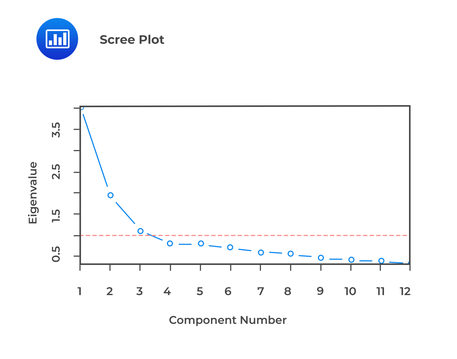
The scaled covariance gives the explanatory power of each component. To choose which components to retain, we can keep as many components as necessary to ‘explain’ at least 90% of the total variance or use other criteria such as the Scree test. A Scree test involves the examination of a line chart of the variances of each component (called a Scree diagram). The Scree test retains only those principal components before the variances level off, which is easy to observe from the Scree diagram, as shown in the example below:
 We observe that the scree plot levels off after the first three components, this would imply that these three components are enough.
The principal components are combinations of the data set’s original features, making it hard for the analyst to label or directly interpret. Therefore, the end-user of PCA may recognize PCA as something of a “black box.” On the contrary, lower-dimensional datasets make machine learning models quicker for training, reducing overfitting (by avoiding the curse of dimensionality), and are easier to interpret.
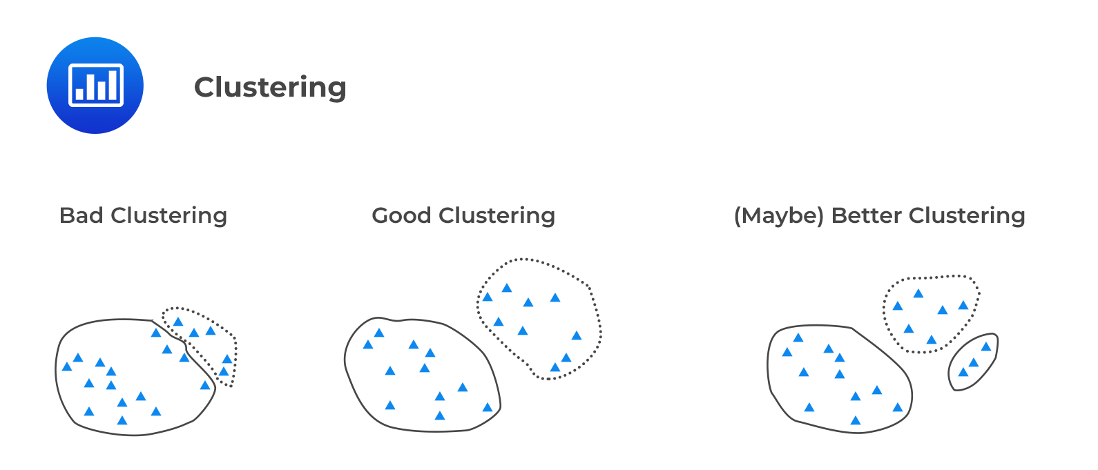
Clustering is used to organize data points into groups called clusters. A good cluster has observations that are similar or close to each other inside the cluster, a property called cohesion, but dissimilar observations between clusters, a property called separation.
The following figure illustrates intra-cluster cohesion and inter-cluster separation.
 2.1 K-Means Clustering
K-means algorithm is an iterative algorithm that starts with an initial division of the data into K clusters. It then adjusts that division in a series of steps to increase similarities within each cluster and to increase the heterogeneity between clusters.
The algorithm follows the following steps when performing K-means Clustering:
The k-means algorithm continues to iterate until there is no need to recalculate new centroids. The algorithm has then converged and has minimized intra-cluster distance, thus maximizing cohesion and separation.
One limitation of the k-means algorithm is that it does not guarantee to find the optimal set of clusters because it incorporates a random element. In other words, the hyperparameter, K, must be decided before running the k-means algorithm.
Finally, the k-means algorithm is applicable in investment practice, particularly in data exploration for discovering patterns in high-dimensional data or as a method for deriving alternatives to existing static industry classifications.
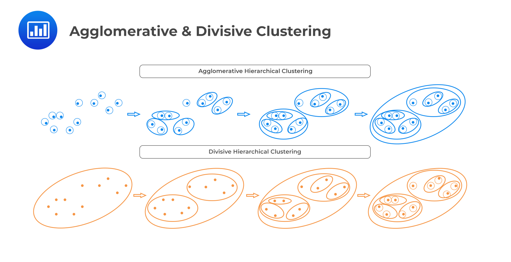
Hierarchical clustering is an unsupervised iterative algorithm used to build a hierarchy of clusters. In hierarchical clustering, the algorithms create transitional rounds of clusters of increasing (i.e., “agglomerative”) or decreasing (i.e., “divisive”) size until a final clustering is reached.
Agglomerative clustering is a bottom-up approach. Each observation begins in its cluster and then merges with other clusters iteratively until all clusters are clumped into a single cluster.
Divisive clustering is a top-down approach. It begins with all the observations belonging to a single cluster. The observations are then split into two clusters based on some similarity or some measure. The algorithm then progressively partitions the intermediate clusters into smaller clusters until each cluster contains only 1 observation.
The following figure demonstrates both agglomerative and divisive clustering:

Question
Hierarchical clustering is most likely to be described as an approach in which:
A. Grouping of observations is unsupervised.
B. Features are grouped into a pre-specified number, k, of clusters.
C. Observations are classified according to predetermined labels.
Solution
A is correct.
Hierarchical clustering is an unsupervised ML algorithm. The implication is that the grouping of observations is unsupervised.
B is incorrect. It refers to k-means clustering.
C is incorrect. It describes classification, which involves supervised learning.
Reading 6: Machine Learning
LOS 6 (d) Describe unsupervised machine learning algorithms—including principal components analysis, K-means clustering, and hierarchical clustering—and determine problems for which they are best suited
Get Ahead on Your Study Prep This Cyber Monday! Save 35% on all CFA® and FRM® Unlimited Packages. Use code CYBERMONDAY at checkout. Offer ends Dec 1st.