Supervised Machine Learning Algorithms

1. Penalized Regression

Penalized regression is a technique that is useful for reducing/shrinking a large number of features to a manageable set and for making good predictions in a variety of large data sets. It is used to avoid overfitting. Models in which each variable plays an essential role tend to work well in prediction because they are less subject to overfitting.

The penalized regression allows us to create a linear regression model that is penalized for having too many variables in the model by adding a constraint in the equation. This is through shrinkage or regularization methods.

An excellent example of penalized regression is LASSO regression.

1.1. LASSO Regression

LASSO (least absolute shrinkage and selection operator) contracts the regression coefficients toward zero. The shrinking is done by penalizing the regression model with a penalty term, known as the L1 norm, which is the sum of the absolute coefficients.

$$ \text{Penalty Term} =\lambda \sum_{k-1}^{K}|\widehat{{b}_{k}}| $$

With \(\lambda>0\).

LASSO also involves minimizing the sum of the absolute values of the regression coefficients as in the following expression:

$$=\sum_{i=1}^{n}(Y_i-Y_{i})^2+\lambda \sum_{k=1}^{K}|\widehat{{b}_{K}}|$$

When \(\lambda=0\), the penalty term reduces to zero, so there is no regularization, and the regression is equivalent to an ordinary least squares (OLS) regression.

The higher the number of variables with non-zero coefficients, the larger the penalty term. Penalized regression, therefore, ensures that a feature is included if the sum of squared residuals declines by more than the penalty term increases. Additionally, LASSO automatically performs feature selection since it eliminates the least essential features from the model.

Lambda is the tuning parameter that decides how much we want to penalize the flexibility of our model. As the value of \(\lambda\) rises, the value of coefficients reduces and thus reducing the variance, consequently avoiding overfitting.

Regularization refers to methods that reduce statistical variability in big dimensional data estimation problems. In this case, reducing regression coefficient estimates toward zero and thereby avoiding complex models and the risk of overfitting.

2. Support Vector Machine

Support vector machine (SVM) is an algorithm technique used for classification, regression, and outlier detection.

Starting with a set of training examples that belong to two specified categories, an SVM model can assign new examples to each category. In essence, the model can “train”  and subsequently predict where a new set of examples belong. The SVM model works by establishing a hyperplane between the two categories that is wide as possible to simplify the prediction process. The model assumes that the data is linearly separable.

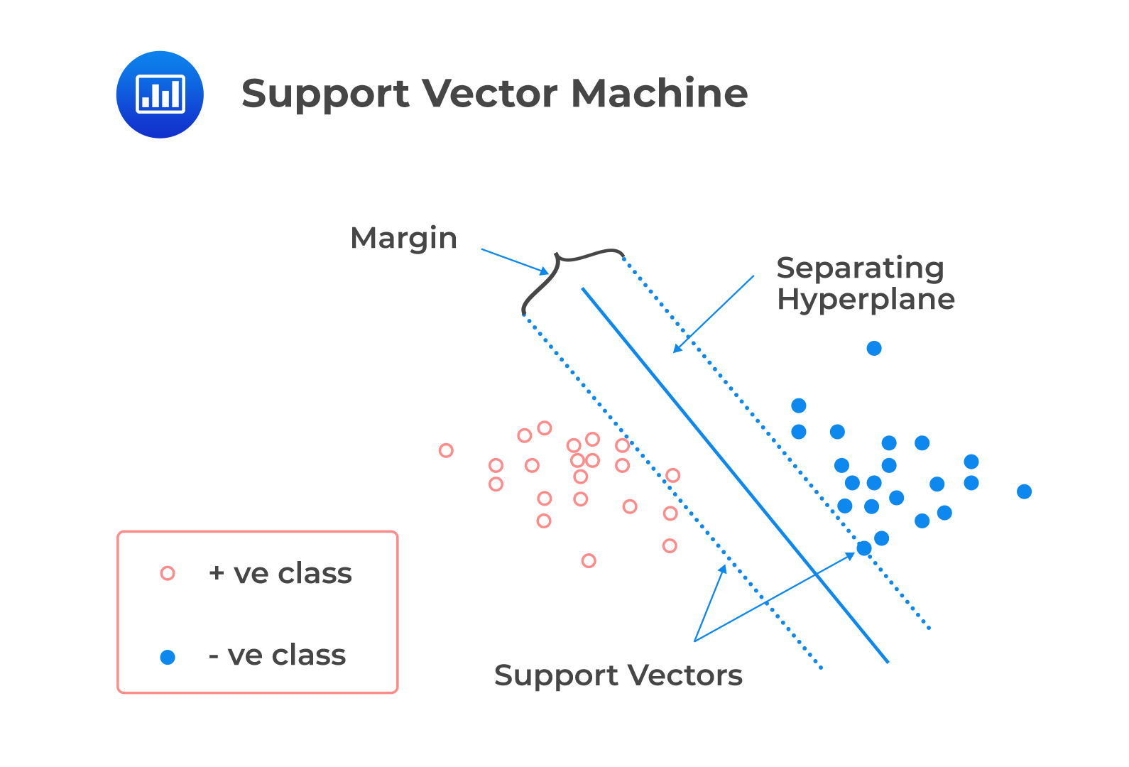A linear classifier is a binary classifier that makes its classification decision based on a linear combination of the features of each data point. SVM is a linear classifier that determines the decision boundary that optimally separates the observations into two sets of data points. The decision boundary is a hyperplane if the data has more than three dimensions. SVM solves the optimization problem so that:

• Support vectors have the shortest possible distance from the separating hyperplane or the boundary.
• The two classes lie on separate sides of the hyperplane.

SVM can be applied to corporate financial statements or bankruptcy databases as they are complex high-dimensional data sets. It is essential to note that training the SVM algorithm is time-consuming, and the algorithm structure is challenging to understand.

3. K-Nearest Neighbor

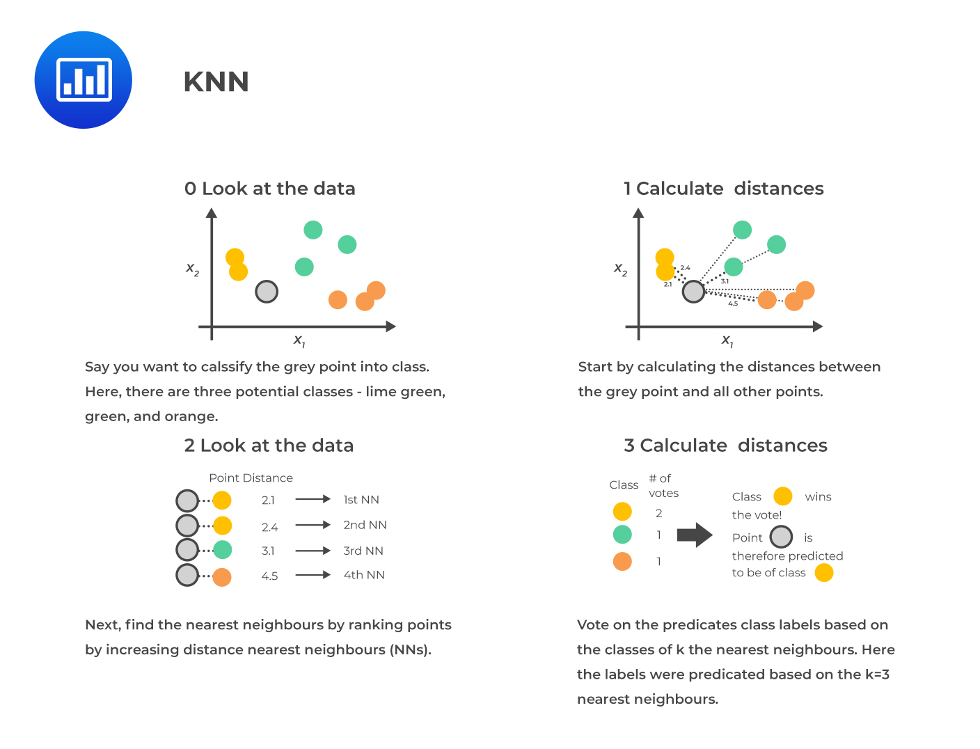
K-nearest neighbor (KNN) is an algorithm used for classification and regression. The idea is to classify a new observation by finding similarities (“nearness”) between it and its k-nearest neighbors in the existing data set.

Example of KNN

In KNN, K is the number of the nearest neighbors, which is the core deciding factor. The simplest case is when K = 1; in this case, the algorithm is known as the nearest neighbor algorithm.

KNN is a straightforward, intuitive model that is still very powerful because it is non-parametric; the model makes no assumptions concerning the distribution of the data. Further, it can be employed for multiclass classification.

The main challenge facing KNN is the definition of “near.” Additionally, an important decision relates to the distance metric used to model nearness because an inappropriate measure generates poorly performing models. More subjectivity may arise depending on the correct choice of the correct distance measure. KNN can be applied in the investment industry, including bankruptcy prediction, stock price prediction, corporate bond credit rating assignment, and customized equity and bond index creation.

4. Classification and Regression Tree

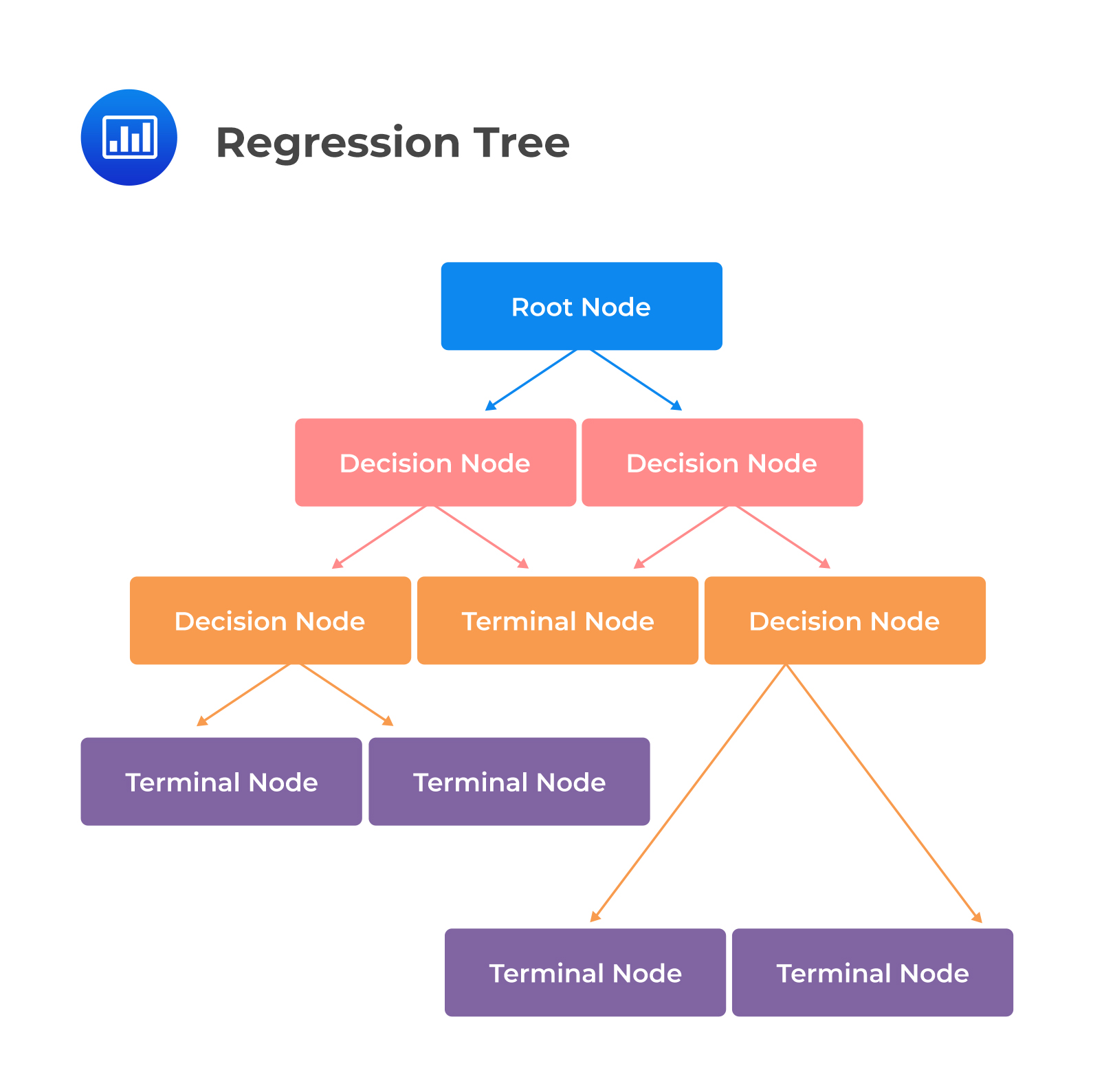
Classification and Regression Tree (CART), also known as a decision tree, is most commonly applied to binary classification or regression. Items are classified by asking a series of questions that home in on the most likely classification. It is essential to avoid overfitting by applying a stopping criterion or by pruning the decision tree. At each node, the algorithm chooses the feature and the cutoff value for the selected feature that generates the most extensive separation of the labeled data to minimize classification error.

Suppose we want to predict if a stock is an attractive investment or a value trap, i.e., an investment that is likely to be unprofitable but cheaply priced. High profitability is only relevant if the stock is cheap. For example, in this hypothetical case, if P/E is less than 20, leverage is high (debt to total capital > 50%), and sales are expanding (sales growth > 20%). Multiple linear regression fails typically in situations where the relationship between the features and the outcome is non-linear.

The decision tree to determine if the investment is attractive or a value trap is as follows:

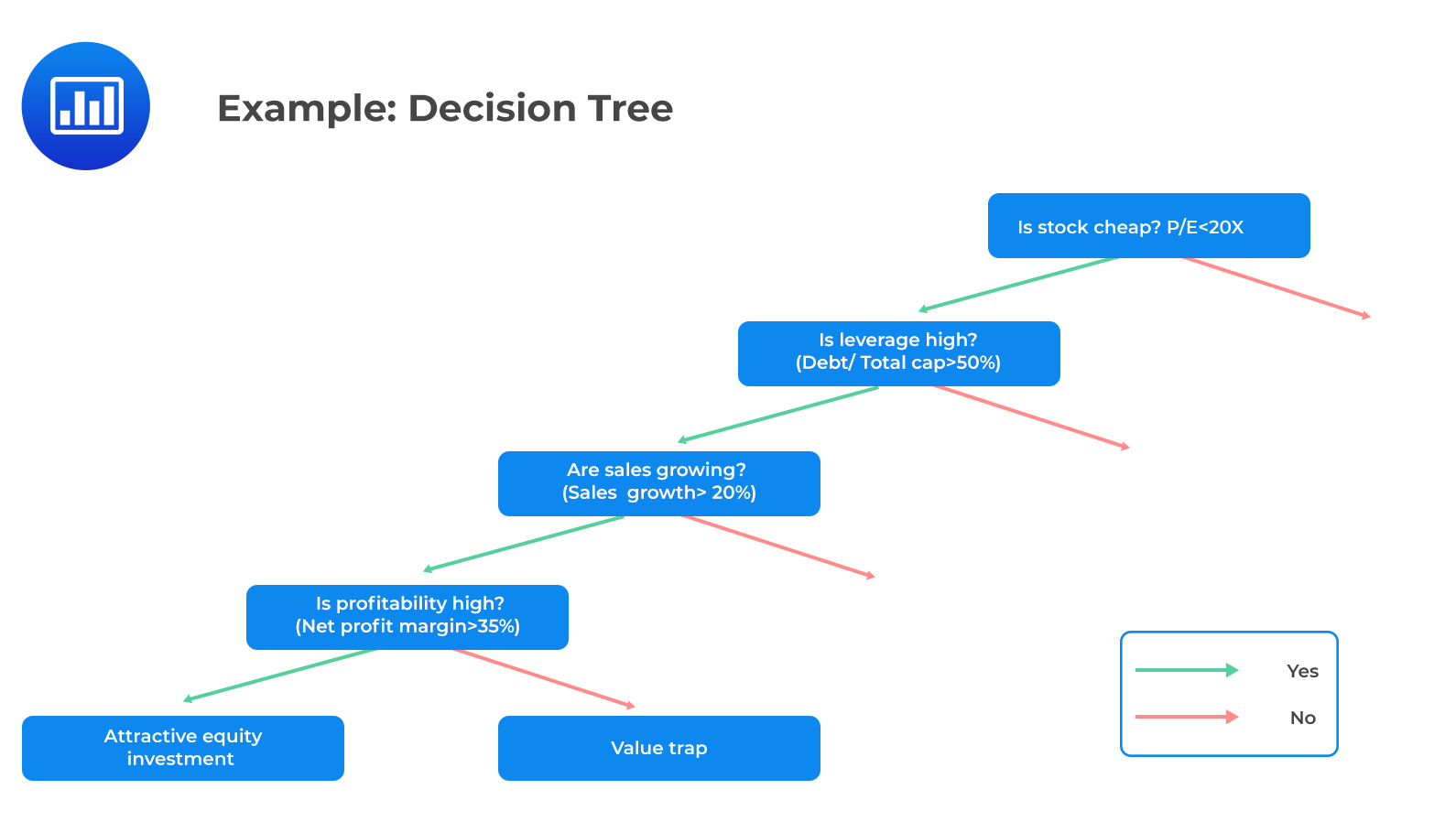The tree in the CART provides a visual explanation for prediction. Moreover, it is a powerful tool to build expert systems for decision-making processes. It can induce robust rules despite noisy data and complex relationships between high numbers of features.

CART can be applied in enhancing fraud detection in financial statements, generating consistent decision processes in equity and fixed-income selection, and simplifying the communication of investment strategies to clients.

5. Ensemble Learning and Random Forest

Ensemble learning is the technique of combining the predictions from a collection of models, whereas the combination of multiple learning algorithms is known as the ensemble method. Ensemble learning produces more accurate and more stable predictions than any other single model typically. Ensemble methods aim to decrease variance (bagging), decrease bias (boosting), and improve predictions (stacking).

Ensemble learning can be divided into two main categories:

• A homogeneous ensemble is a combination of the same algorithm, using different training data that are based on say a bootstrap aggregating technique.
• A heterogeneous ensemble entails different types of algorithms combined with a voting classifier.

5.1. Voting Classifiers

Voting works by first creating two or more individual ML models from your training data set. A voting classifier is then used to combine results of the models and average predictions of the sub-models when tasked to make predictions for new data. A majority-vote classifier can also be used to assign to a new data point the predicted label with the most votes.

It is crucial to look for diversity in the choice of algorithms, modeling techniques, and hypotheses to mitigate the risk of overfitting.

5.2. Bootstrap Aggregating

Bootstrap aggregation, also known as bagging, involves taking multiple samples from the training dataset with replacement and training the algorithm. The final output prediction is obtained by aggregating the n predictions using a majority-vote classifier for classification or an average for a regression. Bagging improves the stability of predictions and protects against overfitting the model.

5.3. Random Forest

Random forest, like its name suggests, comprises of a large number of individual decision trees that operate as an ensemble. Training dataset samples are taken with replacement, but the trees are constructed in a way that reduces the correlation between individual classifiers. The fundamental concept here is that a large number of arguably uncorrelated models or trees operating as a group outperform any of the individual constituent models.

A simple illustration of random forest is as follows:

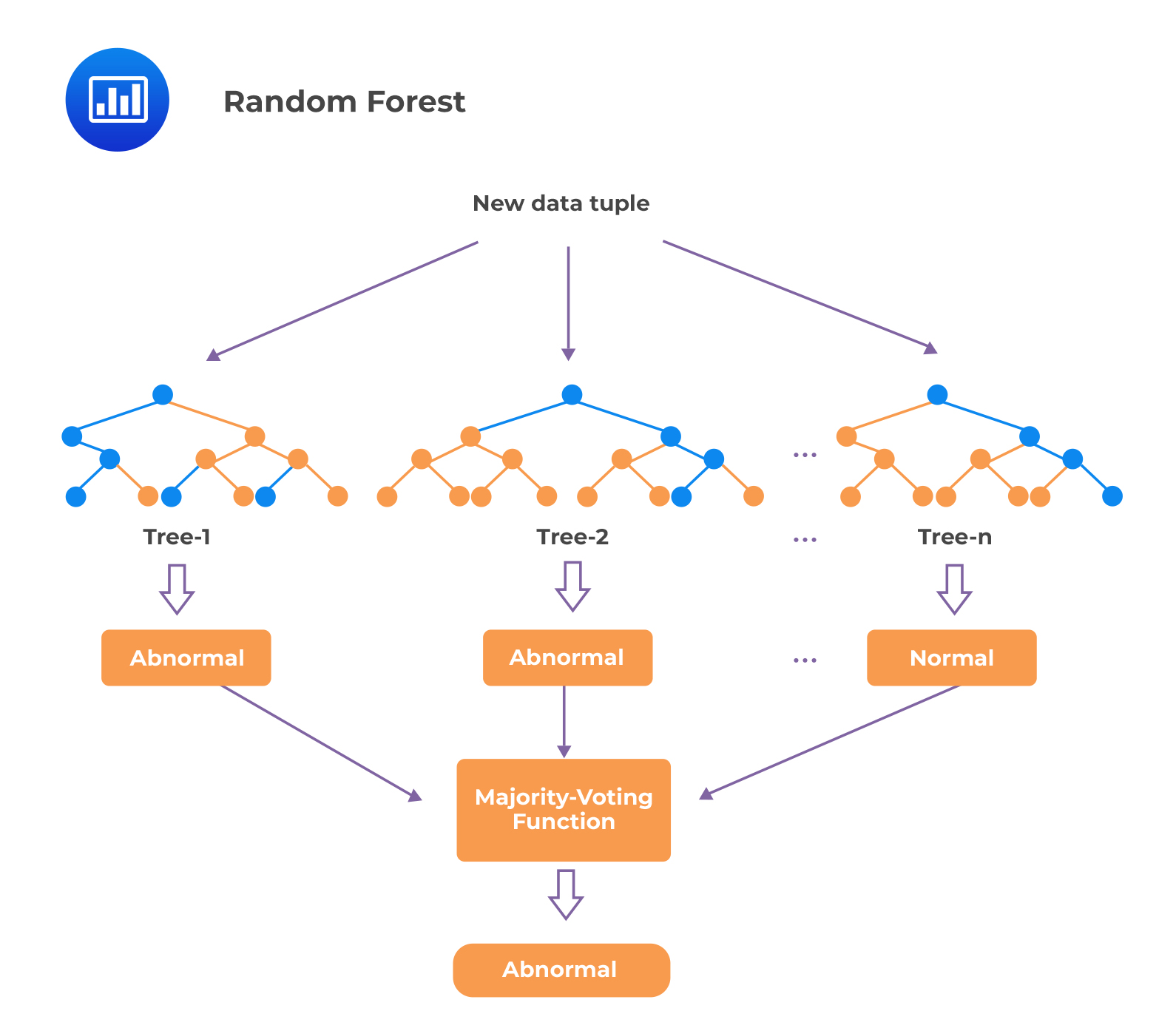The process involved in random forest reduces the risk of overfitting on the training data. It also reduces the ratio of noise to signal because errors cancel out across the collection of slightly different classification trees. However, a significant drawback of random forest is that it lacks the ease of interpretability of individual trees; as a result, it is considered a relatively black box-type algorithm.

Random forest is a robust algorithm that can be applied in many investment aspects. For example, use in factor-based investment strategies for asset allocation and investment selection.

Question

An investment analyst wants to employ ML techniques to upgrade the way she selects her stock investments. She decides to employ machine learning to divide her investable universe of 2,000 stocks into 8 different groups, based on a wide variety of the most relevant financial and non-financial characteristics. The aim is to mitigate unintended portfolio concentration by selecting stocks from each of these distinct groups.

Assuming she utilizes regularization in the ML technique, which of the following ML models is least likely appropriate?

1. Regression tree with pruning
2. LASSO with \(\lambda\) equal to 0
3. LASSO with \(\lambda\) between 0.5 and 1

Solution

The correct answer is B.

Recall that with LASSO, \(\lambda\) is the penalty term. When the penalty term reduces to zero, there is no regularization, and the regression resembles an ordinary least squares (OLS) regression. Therefore, LASSO with \(\lambda\) equal to 0 will be the least appropriate.

A is incorrect. One way of regularization in a decision tree or CART is through pruning. Pruning reduces the size of the regression tree—sections that provide little explanatory power are eliminated or pruned.

C is incorrect. LASSO with \(\lambda\) between 0.5 and implies a reasonably significant penalty term. It, therefore, requires that a feature makes an adequate contribution to model fit to offset the penalty from including it in the model.

Reading 6: Machine Learning

LOS 6 (c) Describe supervised machine learning algorithms—including penalized regression, support vector machine, k-nearest neighbor, classification and regression tree, ensemble learning, and random forest—and determine the problems for which they are best suited