


Valuation of Equities and Currencies U ...
Some underlying instruments have carry benefits. These benefits include dividends for stock options,... Read More

Machine learning (ML) model training entails three tasks: method selection, performance evaluation, and tuning. While there are no standard rules for training an ML model, having a fundamental understanding of domain-specific training data and ML algorithm principles is key to proper model training.
Recall that in the previous stages, we have transformed unstructured text data into forms of data matrixes or tables for machine training. Therefore, the ML model training for structured and unstructured data is typically similar. In ML model training, all we are doing is fitting a system of rules on a training dataset to establish data patterns. Model training steps are as follows:
The first step of the training process is selecting and applying an algorithm to an ML model. The following factors determine method selection:
It is vital to note that more than one method can be used to exploit the advantages of each method. Additionally, before model training begins, the master data set is split into three subsets in case of supervised learning. The figure below demonstrates a possible way of splitting the data.
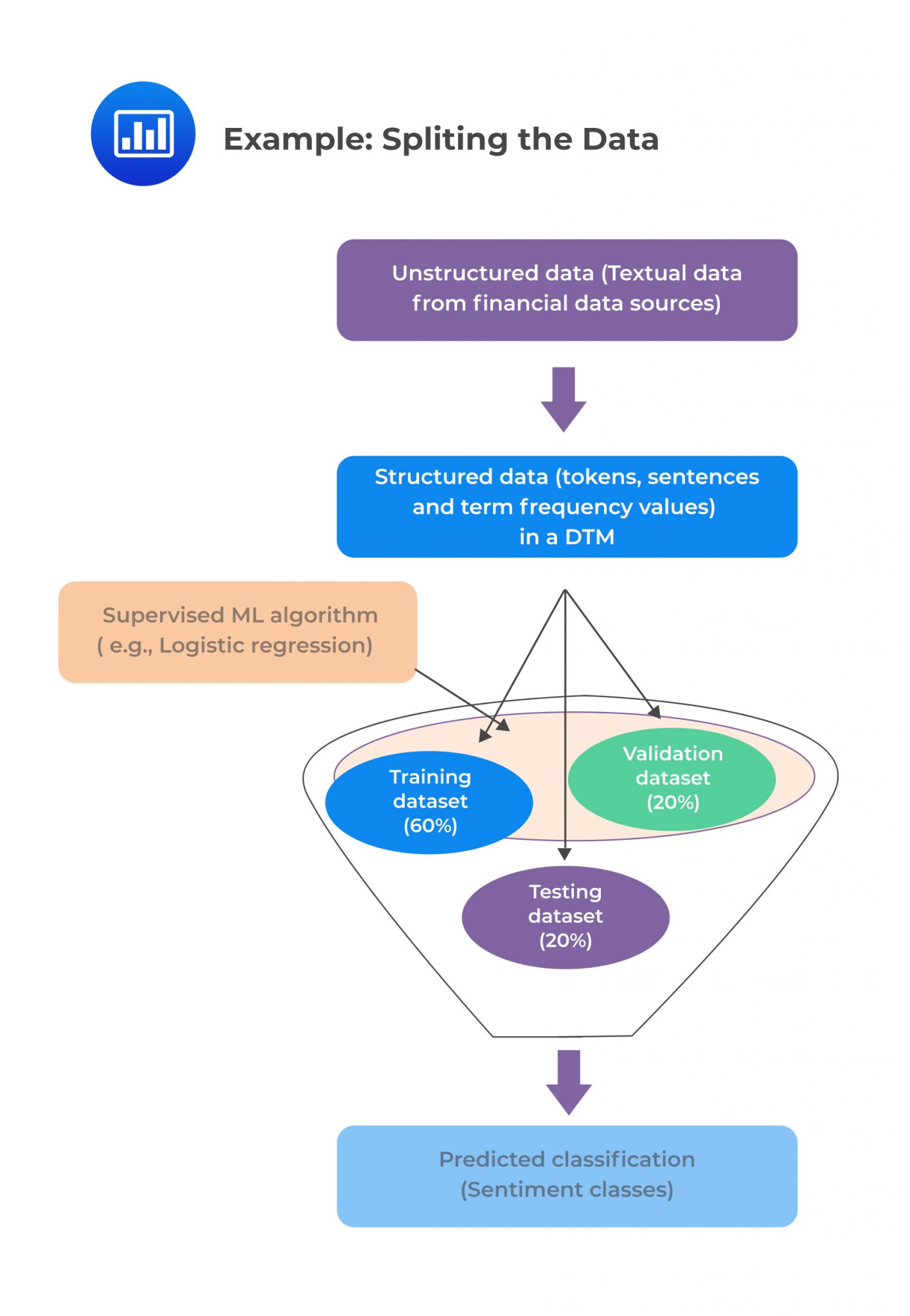 For unsupervised learning, no splitting is needed due to the absence of labeled training data.
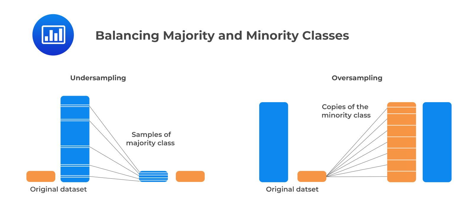
In some cases, the number of observations for a particular class may be significantly larger than for other classes. This is known as class imbalance, and it is linked to data used in supervised learning. Resampling the data set solves this problem. Undersampling and oversampling approaches apply to balancing the classes.
Undersampling works by reducing the majority class (“0”). This method is applicable when the quantity of data is adequate. By keeping all samples in the minority class (“1”) and randomly selecting an equal number of samples in the majority class, a balanced new dataset can be retrieved for further modeling.
Oversampling, on the contrary, is used when the quantity of data is not sufficient. Its goal is to balance the dataset by increasing the size of the minority samples. Instead of getting rid of majority samples, new minority samples are generated using, say repetition, and bootstrapping.
The following figure shows the idea of balancing the majority and the minority classes.
 2. Performance Evaluation
Performance evaluation of the model training is essential for validation of the model. In this section, we discuss the various techniques appropriate for measuring model performance. For simplicity, we will mostly deal with binary classification models.
Error analysis entails four basic evaluation metrics: true positive (TP), false positive (FP), true negative (TN), and false-negative (FN) metrics. FP is also known as Type I error, whereas FN is also called a Type II error. The confusion matrix below gives a better visualization of these metrics:
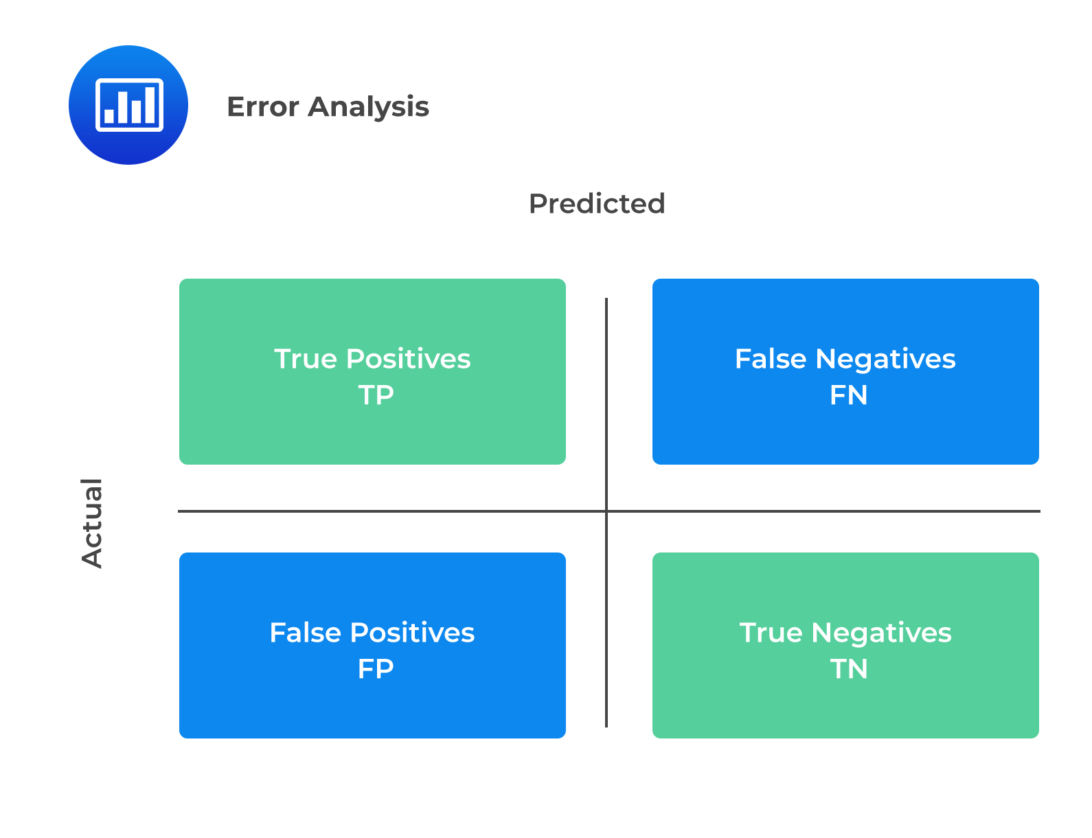 The explanation of the terms in the confusion matrix is as follows:
Precision (P) is the proportion of correctly predicted positive classes to total predicted positive classes. Precision is useful in situations where the cost of false positives (FP), or Type I error is high.
$$\text{Precision (P)}=\frac{\text{TP}}{\text{TP}+\text{FP}}$$
Recall (sensitivity) is the proportion of correctly predicted positive classes to the total actual positive classes. It is useful where the cost of FN or Type II error is high.
$$\text{Recall (R)}=\frac{\text{TP}}{\text{TP}+\text{FN}}$$
Accuracy is the percentage of correctly predicted classes out of total predictions. It is a standard metric for evaluating model performance. However, it is not a clear indicator of the performance and can generate worse results, especially if the classes are imbalanced.
$$\text{Accuracy}=\frac{\text{TP}+\text{TN}}{\text{TP}+\text{FP}+\text{TN}+\text{FN}}$$
FI score is the harmonic mean of precision and recall. F1 score is more appropriate than accuracy when there is a class imbalance in the dataset, and it is necessary to measure the equilibrium of precision and recall. The higher the F1 score, the better the model performance.
$$\text{F1 score}=\frac{(2\times\text{Precision}\times\text{Recall})}{\text{Precision}+\text{Recall}}$$
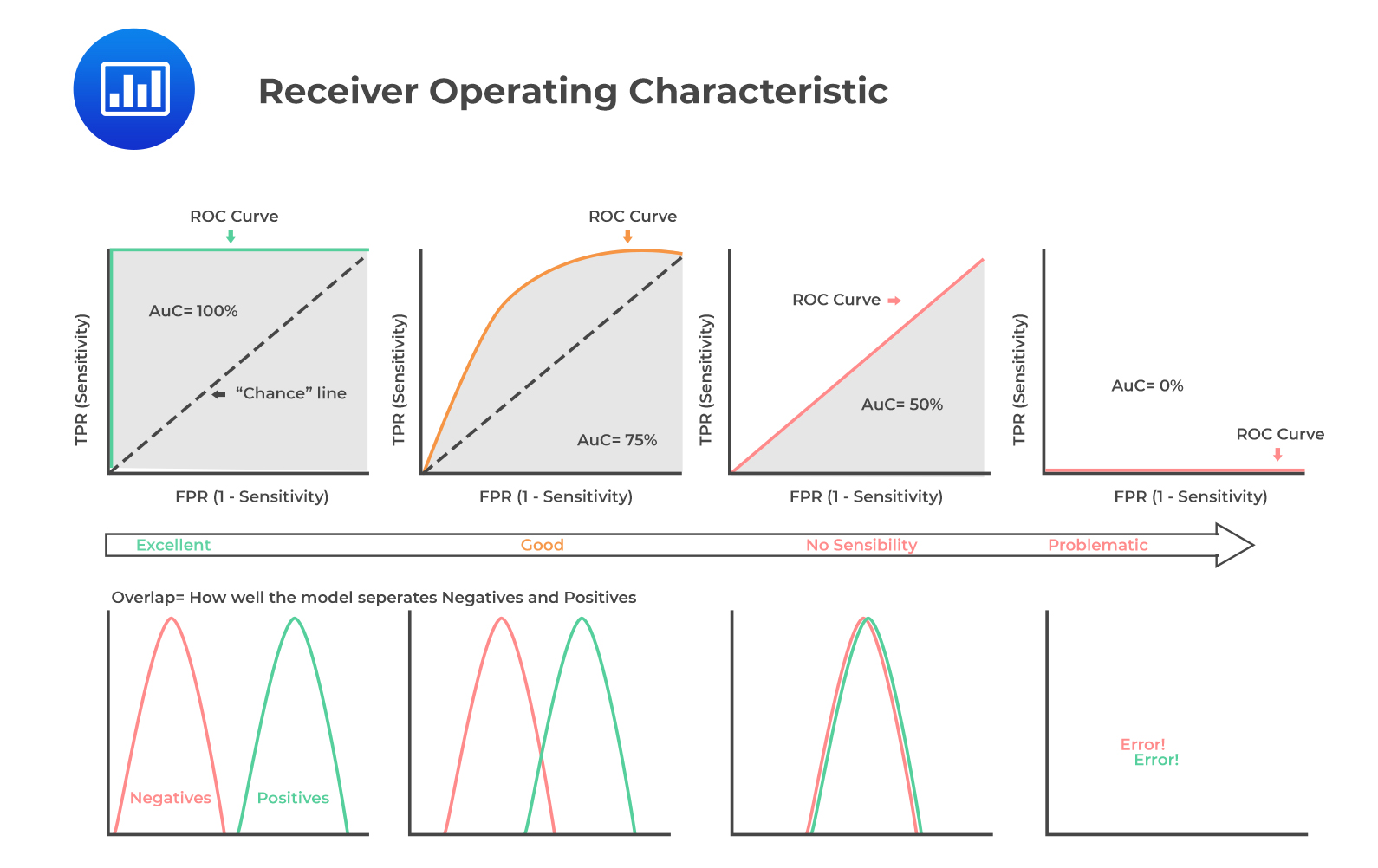
ROC involves plotting a curve showing the trade-off between the false positive rate (x-axis) and true positive rate (y-axis) for various cutoff points where:
$$\text{False positive rate (FPR)}=\frac{\text{FP}}{\text{TN}+\text{FP}}$$
And,
$$\text{True positive rate (TPR)}=\frac{\text{TP}}{\text{TP}+\text{FN}}$$
As TPR increases, FPR also increases. Furthermore, a more convex curve indicates better model performance. AUC is equivalent to the area under the ROC curve. The higher the numerical value of AUC, the better the prediction.
The following figure demonstrates all you need to know about ROC curves and AUCs:
 c. Root Mean Squared Error (RMSE)
RMSE is a single metric that captures all the prediction errors in the data (n). It is appropriate for continuous data prediction and is mostly used for regression methods.
$$\text{RMSE}=\sqrt{\sum_{i=1}^{n}\frac{(\text{Predicted}_{i}-\text{Actual}_{i})}{n}}$$
A small RMSE indicates potentially better model performance.
The main objective of tuning is to improve model performance. Model-fitting has two types of error: bias and variance. Bias error emerges when the model is underfitted, whereas variance error is associated with overfitting. Both errors can be reduced, so the total aggregate error (bias error + variance error) is at a minimum. The bias-variance trade-off is vital to finding an optimum balance where a model neither underfits nor overfits.
Tuning is usually a trial-and-error process. It entails a continuous change of some hyperparameters. The algorithm is then run on the data again, and the output is compared to its performance using the validation set. This determines the set of hyperparameters, which results in the most accurate model. This method is known as a grid search.
A fitting curve of the training sample error and cross-validation sample error on the y-axis versus model complexity on the x-axis is useful for managing the bias vs. variance error trade-off. Fitting curves visually aid in tuning hyperparameters.
The following figure shows a bias-variance error trade-off by plotting a generic fitting curve for hyperparameter:
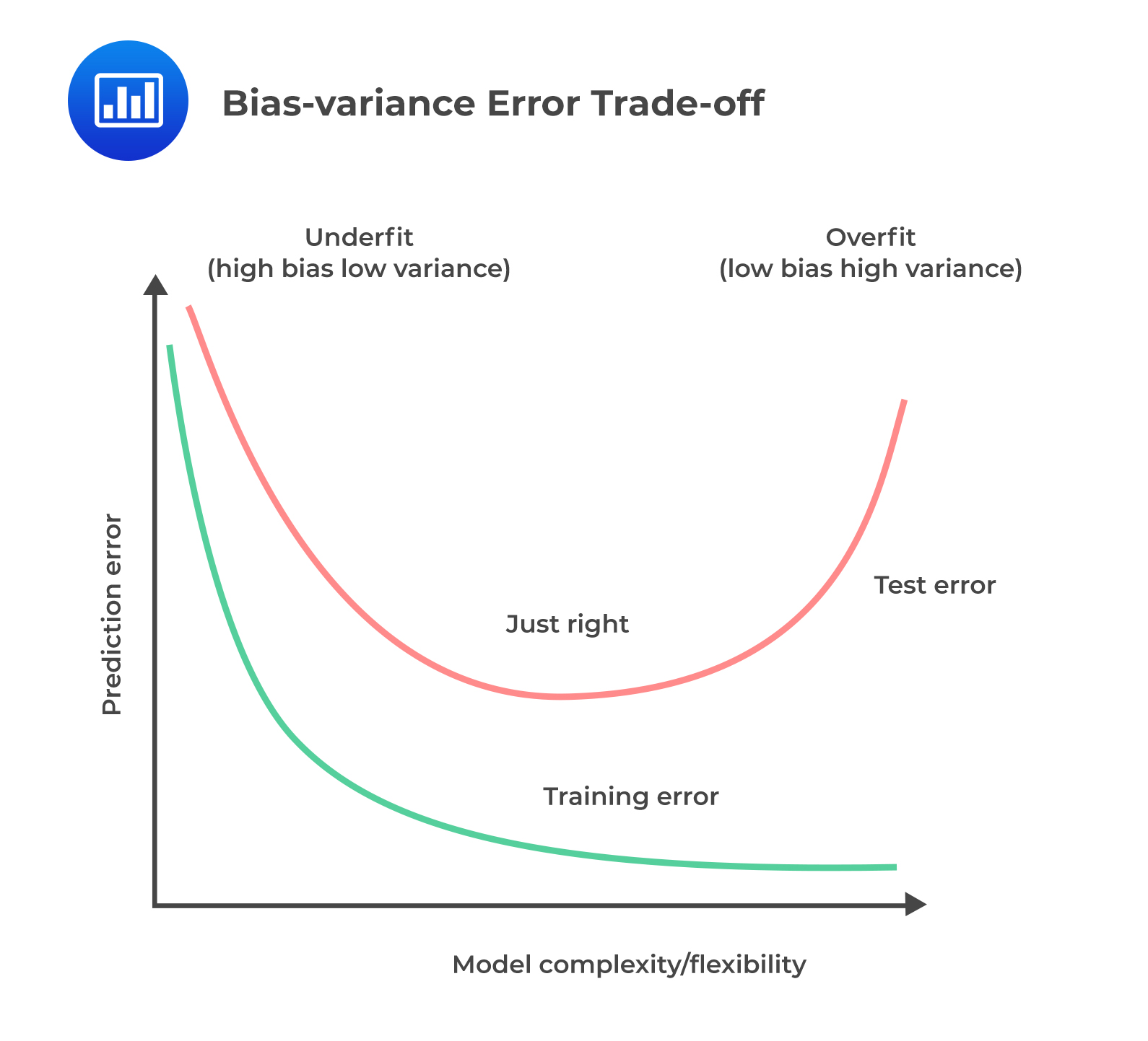 If there exists a high bias or variance even after the tuning of hyperparameters, a large number of training observations (instances) may be needed. Additionally, the number of features included in the model may need to be reduced in the case of high variance or increased in the case of high bias. The model then needs to be re-trained and re-tuned using the new training dataset.
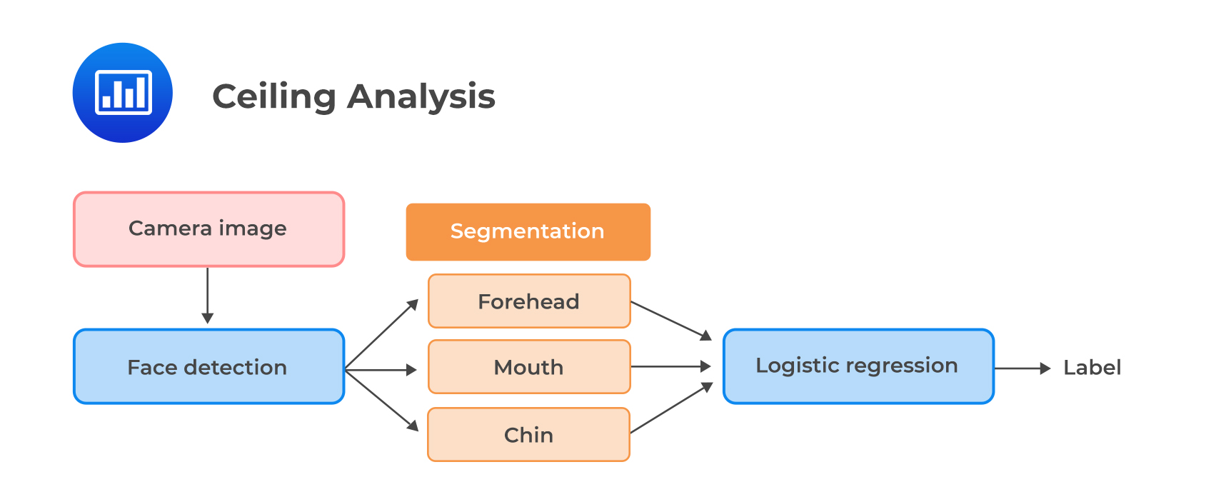
Ceiling analysis is employed in the case of a complex model, i.e., where a large model is comprised of sub-model(s). Ceiling analysis is a systematic process of assessing different components in the pipeline of model building. It assists in understanding the part of the pipeline that can potentially improve in performance by further tuning.
 Question
Amelia Parker is a junior analyst at ABC Investment Ltd. Parker is building a model that has an improved predictive power. She plans to improve the existing model that purely relies on structured financial data by incorporating finance-related text data derived from news articles and tweets relating to the company. After preparing and wrangling the raw text data, Parker performs exploratory data analysis. She creates and analyzes a visualization that shows the most informative words in the dataset based on their term frequency (TF) values to assist in feature selection.
Once satisfied with the final set of features, Parker selects and runs a model on the training set that classifies the text as having positive sentiment (Class “1”) or negative sentiment (Class “0”). She then evaluates its performance using error analysis. The resulting confusion matrix is as follows:
Confusion Matrix
$$\small{\begin{array}{l|l|l|l} {}&{} & \text{Actual Training Results}\\ \hline{}& {}& \text{Class “1”} & \text{Class “0”}\\ \hline\text{Predicted Results} & \text{Class “1”} & \text{TP=200} & \text{FP=70}\\ {}& \text{Class “0”} & \text{FN=40} & \text{TN=98}\\ \end{array}}$$
Based on the above confusion matrix, the models F1 score and accuracy metric are most likely to be:
A. 74% and 83%, respectively.
B. 74% and 78%, respectively.
C. 78% and 73%, respectively.
Solution
The correct answer is C.
The model’s F1 score, which is the harmonic mean of precision and recall, is computed as:
$$\text{F1 score}=\frac{(2\times \text{Precision}\times\text{Recall})}{\text{Precision}+\text{Recall}}$$
$$\text{Precision (P)}=\frac{\text{TP}}{\text{TP}+\text{FP}}$$
$$\begin{align*}\text{Precision (P)}&=\frac{200}{200+70}\\&=74\%\end{align*}$$
$$\text{Recall (R)}=\frac{\text{TP}}{\text{TP}+\text{FN}}$$
$$\begin{align*}\text{Recall (R)}&=\frac{200}{200+40}\\&=83\%\end{align*}$$
$$\text{F1 score}=\frac{(2\times \text{Precision}\times\text{Recall})}{\text{Precision}+\text{Recall}}$$
$$\begin{align*}\text{F1 score}&=\frac{(2\times74\times83)}{74+83}\\&=78\%\end{align*}$$
The model’s accuracy, which is the proportion of correctly predicted classes out of total predictions, is solved as follows:
$$\text{Accuracy}=\frac{\text{TP}+\text{TN}}{\text{TP}+\text{FP}+\text{TN}+\text{FN}}$$
$$\begin{align*}\text{Accuracy}&=\frac{200+98}{200+70+98+40}\\&=73\%\end{align*}$$
Reading 7: Big Data Projects
LOS 7 (d) Describe objectives, steps, and techniques in model training
Offered by AnalystPrep


Get Ahead on Your Study Prep This Cyber Monday! Save 35% on all CFA® and FRM® Unlimited Packages. Use code CYBERMONDAY at checkout. Offer ends Dec 1st.