The Value of Common Shares using Multiperiod Models

Two-Stage Dividend Discount Model

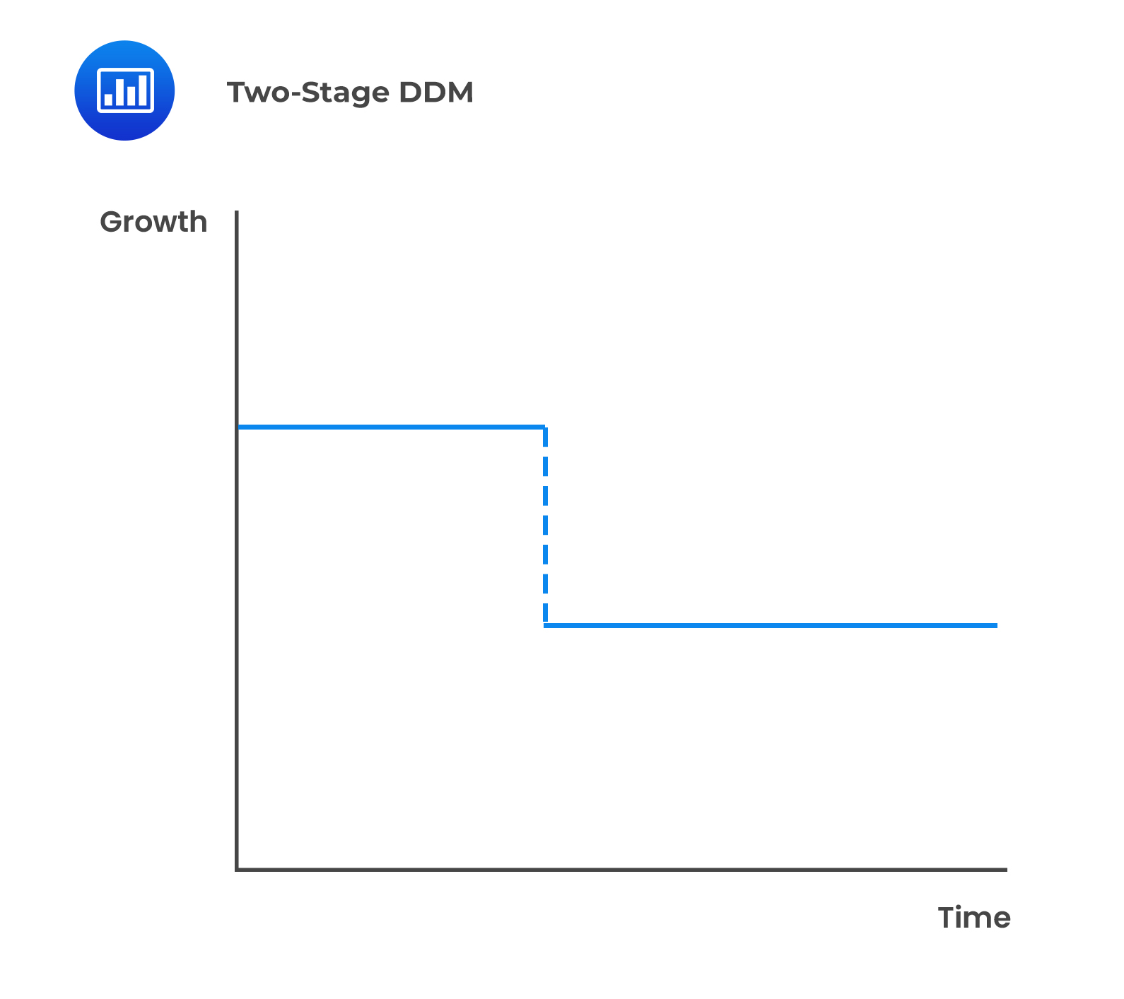
There are two approaches to the two-stage dividend discount model:

i. The General Two-Stage Model

Under this model, a company’s growth is divided into two sections—one where it experiences high growth and the second where its growth is stable and sustainable. The transition from the first stage to the second is abrupt and immediate.

$$\text{V}_0= ∑_{(\text{t}=1)}^{\text{n}}\frac{\text{D}_0(1+\text{g}_{\text{S}})^\text{t}}{(1+\text{r})^\text{t}} +\frac{\text{D}_0 (1+\text{g}_{\text{S}})^\text{n}(1+\text{g}_{\text{L}})}{(1+\text{r})^\text{n}(\text{r}-\text{g}_{\text{L}})}$$

Where:

\(\text{g}_{\text{S}}=\) Short-term high growth rate.

\(\text{g}_{\text{L}}=\) Long-term sustainable growth rate.

\(\text{r}=\) Required rate of return.

\(\text{n}=\) Length of the extraordinary growth rate.

Example: Two-Stage Model

ABC’s current dividend of $0.50 is expected to grow by 8% per year for the next 3 years. Thereafter, the dividend growth rate will decline to 5% and remain at that level indefinitely. Using a required rate of return of 13%, its share price value would be calculated as:

$$\begin{align*}\text{V}_0&= ∑_{(\text{t}=1)}^{\text{n}}\frac{\text{D}_0(1+\text{g}_{\text{S}})^\text{t}}{(1+\text{r})^\text{t}} +\frac{\text{D}_0 (1+\text{g}_{\text{S}})^\text{n}(1+\text{g}_{\text{L}})}{(1+\text{r})^\text{n}(\text{r}-\text{g}_{\text{L}})}\\ \\  \text{D}_{1}&=$0.50\times1.08=$0.54\\ \text{D}_{2}&=$0.54\times1.08=$0.583\\ \text{D}_{3}&=$0.583\times1.08=$0.630\\ \text{D}_{4}&=$0.630\times1.05=$0.662\\\text{V}_{3}&=\frac{0.662}{13\%-5\%}=$8.275\\ \\ \text{V}_{0}&=\frac{0.54}{1.13}+\frac{0.583}{(1.13)^{3}}+\frac{0.63+8.275}{(1.13)^{3}}=7.10\end{align*}$$

Interpretation of the General Two-Stage DDM

1. The present value (PV) of the terminal value (at the end of year 3) is \(\frac{$8.275}{(1.13)^{3}}=$5.73\).
2. The PV of the terminal value makes up 80.70% \(\bigg(=\frac{$5.73}{$7.10}\bigg)\) of the total value of the share.
3. Accordingly, the valuation depends more on the growth rate and the required rate of return assumptions in the Gordon’s growth model.

A company may experience supernormal growth for a few periods, after which the growth rate falls to a sustainable level. This may be due to patents, a first-mover advantage, or a factor that gives the company an edge. Subsequently, the growth rate will fall to a sustainable level. As such, a different discount rate may be used for the high-growth stage and the sustainable mature stage to reflect the different levels of risks involved.

A limitation to the general two-stage model is that the transition between the initial supernormal growth period and the sustainable mature growth rate is abrupt and immediate.

Valuing a Non-Dividend Paying Company

A company that is not currently paying any dividends but will begin paying dividends in the future may still be valued using the dividend discount model. To value such a company, an analyst can use a multistage DDM, where the first section’s value equals zero.

On the other hand, suppose a company has no intentions of paying dividends, or it is difficult to predict the timing of dividends. In that case, an analyst can use the free cash flow or residual income model to value the company.

ii. The H-model

Under this model, there are two distinct stages but the transition from the high growth section to the mature stage is smooth and linear.

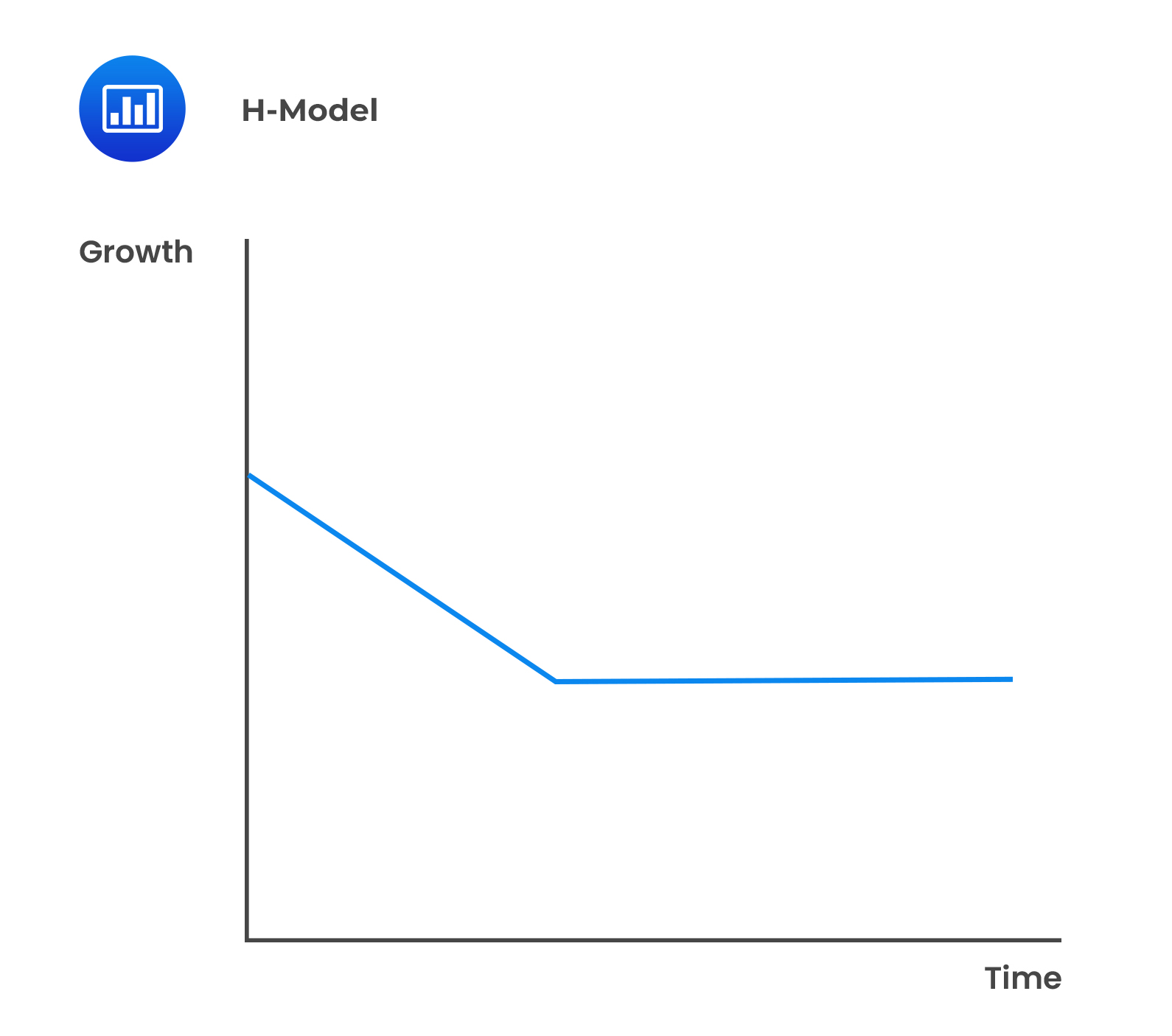The value of a share using the H-model is:

$$\text{V}_0= \frac{\text{D}_0 (1+\text{g}_{\text{L}} )+\text{D}_0\text{H}(\text{g}_{\text{S}}-\text{g}_{\text{L}})}{\text{r}-\text{g}_{\text{L}}}$$

Where:

\(\text{V}_{0}=\) Value per share at \(t = 0\).

\(\text{D}_{0}=\) Current dividends.

\(\text{r}=\) Required rate of return on equity.

\(\text{H} =\) Half-life in years of the high-growth period.

 \(\text{g}_{\text{S}}=\) Initial short term dividend growth rate.

\(\text{g}_{\text{L}}=\) Normal long-term dividend growth rate after the high growth period.

Example: The H-Model

XYZ’s current dividend of $0.80. The current growth of 8% per year is expected to linearly decline to 5% over the next 10 years and after that remain at that level indefinitely. Using a required rate of return of 13%, its share value would be calculated as:

$$\begin{align*}\text{V}_0&= \frac{\text{D}_0 (1+\text{g}_{\text{L}} )+\text{D}_0\text{H}(\text{g}_{\text{S}}-\text{g}_{\text{L}})}{\text{r}-\text{g}_{\text{L}}}\\ \\ &=\frac{0.80(1.05)+0.80(5)(0.03)}{0.08}\\ \\ &=12.0\end{align*}$$

Interpretation of the Two-Stage H-Model

If the normal growth were to commence immediately, the value of the stock would equal \(\frac{D_{0}(1+g_{L})}{r-g_{L}}=\frac{$0.80(1+0.05)}{0.13-0.05}=$10.50\). The extraordinary growth adds $1.50 to the share’s value.

Three-Stage Dividend Discount Model

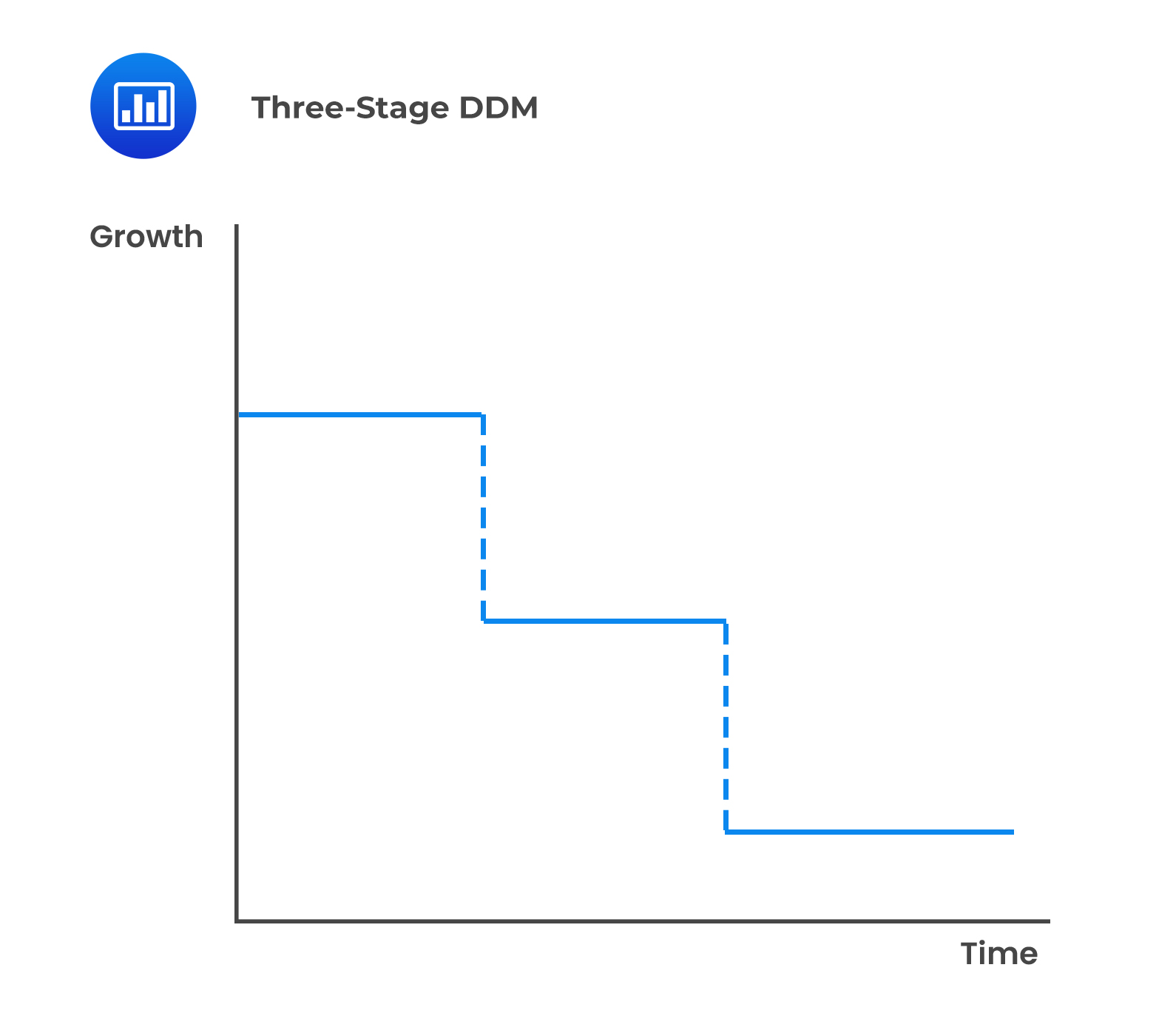
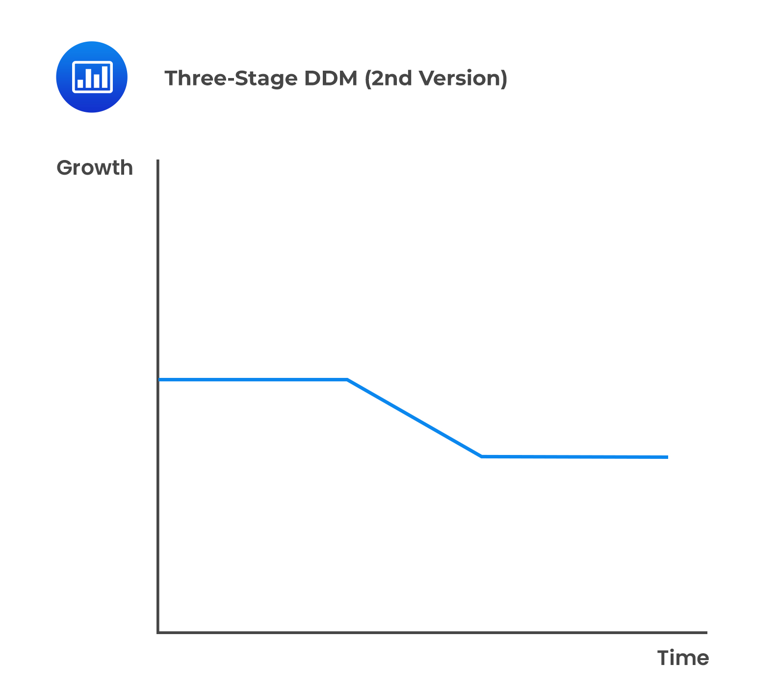
There are two approaches to the three-stage dividend discount model differentiated by the modeling of the second stage:

1. A company has three distinct growth stages, and the second stage’s growth rate is constant. For example, stage 1 could have 20% growth for four years, stage 2 could have 8% growth for five years, and stage 3 could have 4% growth thereafter.
   
2. The growth rate in stage 2 is assumed to decline linearly to the mature, sustainable growth rate. Therefore, stages 2 and 3 are treated as an H-model.
   
   Valuing a company using this model requires the following:
   • Estimate the current dividend.
   • Estimate the length of the first, second, and third stages.
   • Estimate the expected growth rates of the first and third stages.
   • Estimate the required return on equity.
   • Compute the expected dividends and the sum of their present values in stage 1.
   • Apply the H-model to the second and third stages to get the value of the share at the beginning of stage 2.
   • Then, find the present value of the H-model value as of today \((t = 0)\).
   • Finally, sum the present value from stage 1 and the present value of the H-model value.

Example: Three-Stage Dividend Discount Model

Company A recently paid a dividend of $2.00, and it is expected to grow at 14% for the next two years, 12% for the following three years, and 6% thereafter. Therefore, using the three-stage dividend discounted and assuming a required rate of return is 11%, the value of the stock can be estimated as:

$$\begin{align*}\text{D}_1&=\$2×1.14=\$2.28\\ \text{D}_2&=\$2.28×1.14=\$2.60\\ \text{D}_3&=\$2.60×1.12=\$2.91\\ \text{D}_4&=\$2.91×1.12=\$3.26\\ \text{D}_5&=\$3.26×1.12=\$3.65\end{align*}$$

Value of the constant growth dividends:

$$\begin{align*}\text{V}_{5}&=\frac{3.65\times1.06}{11\%-6\%}=77.40\\ \\ \text{V}_0&= \frac{2.28}{(1.11)^1} +\frac{2.60}{(1.11)^2} +\frac{2.91}{(1.11)^3} +\frac{3.26}{(1.11)^4} +\frac{3.63+77.40}{(1.11)^5}\\&=56.52\end{align*}$$

The PV of the terminal value constitutes an overwhelming portion of the total value of the stock, i.e., \(\bigg(81.25\%=\frac{$45.92}{$56.52}\bigg)\).

Question

A company just paid a dividend of $1.50. The dividend is projected to grow at 8% in the next period and linearly decline over the following 6 years to 4% and thereafter remain at that level indefinitely. Using a required rate of return of 10%, the value of the share is closest to:

1. $25.
2. $36.
3. $29.

Solution

The correct answer is C.

$$\begin{align*}\text{V}_0&= \frac{\text{D}_0 (1+\text{g}_{\text{L}} )+\text{D}_0\text{H}(\text{g}_{\text{S}}-\text{g}_{\text{L}})}{\text{r}-\text{g}_{\text{L}}}\\ \\&=\frac{150(1.04)+1.50(3)(0.04)}{0.10-0.04}\\ \\&=29\end{align*}$$

Reading 23: Discounted Dividend Valuation

LOS 23 (l) Calculate and interpret the value of common shares using the two-stage DDM, the H-model, and the three-stage DDM.