Deciphering the Liquidity and Credit C ...
[vsw id=”_sLzMHtACzM” source=”youtube” width=”611″ height=”344″ autoplay=”no”] After completing this reading, you should be... Read More
After completing this reading, you should be able to:
There are two types of distributions, namely parametric and non-parametric distributions. Functions mathematically describe parametric distributions. On the other hand, one cannot use a mathematical function to describe a non-parametric distribution. Examples of parametric distributions are uniform and normal distributions.
Bernoulli distribution is a discrete random variable that takes on values of 0 and 1. This distribution is suitable for scenarios with binary outcomes, such as corporate defaults. Most of the time, 1 is always labeled “success” and 0 a “failure.”
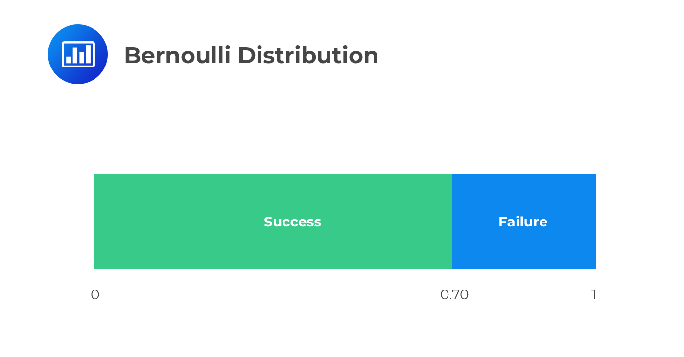 The Bernoulli distribution has a parameter p which is the probability of success, i.e., the probability that X=1, then:
$$ P\left[ X=1 \right] =p\quad and\quad P\left[ X=0 \right] =1-p $$
The probability mass function of the Bernoulli distribution stated as \(X \sim Bernoulli \left(p \right) \) is given by:
$$f_X \left(x \right) =p^x \left(1-p \right)^{1-x}$$
Therefore, the mean and variance of the distribution are computed as:
The PMF confirms that:
$$ P\left[ X=1 \right] =p\quad and\quad P\left[ X=0 \right] =1-p $$
The CDF of a Bernoulli distribution is a step function given by:
$$F_X (x)=\begin{cases} &0, y<0\\&1-p, 0 ≤ y<1\\&1, y≥1\\\end{cases}$$
Therefore, the mean and variance of the distribution are computed as:
$$ E \left(X \right)=p×1+(1-p)×0=p $$
$$V(X)=E(X^2 )-[E(X)]^2=[p×1^2+(1-p)×0^2 ]-p^2=p(1-p)$$
What is the ratio of the mean to variance for X~Bernoulli(0.75)?
Solution
We know that for Bernoulli Distribution,
$$E(X)=p$$
and
$$V(X)=p(1-p)$$
So,
$$\frac{E(X)}{V(X)}=\frac{p}{p(1-p)}=\frac{1}{0.25}=4$$
Thus, E(X): V(X)=4:1
A binomial distribution is a collection of Bernoulli random variables. A binomial random variable quantifies the total number of successes from an independent Bernoulli random variable, with the probability of success being p and, of course, the failure being 1-p. Consider the following example:
Suppose we are given two independent bonds with a default likelihood of 10%. Then we have the following possibilities:
Let \(X\) represent the number of defaults:
$$ P\left[ X=0 \right] ={ \left( 1-10\% \right) }^{ 2 }=81\% $$
$$ P\left[ X=1 \right] =2\times 10\%\times \left( 1-10\% \right) =18\% $$
$$ P\left[ X=2 \right] ={ 10\% }^{ 2 }=1\% $$
If we possess three independent bonds having a 10% default probability then:
$$ P\left[ X=0 \right] ={ \left( 1-10\% \right) }^{ 3 }=72.9\% $$
$$ P\left[ X=1 \right] ={ 3\times 10\%\times \left( 1-10\% \right) }^{ 2 }=24.3\% $$
$$ P\left[ X=2 \right] ={ 3\times { 10\% }^{ 2 }\times \left( 1-10\% \right) }=2.7\% $$
$$ P\left[ X=3 \right] ={ { 10\% }^{ 3 } }=0.1\% $$
Suppose now that we have \(n\) bonds. The following combination represents the number of ways in which \(k\) of the \(n\) bonds can default:
$$ \left( \begin{matrix} n \\ x \end{matrix} \right) =\frac { n! }{ x!\left( n-x \right) ! } \quad \quad \dots \dots \dots \dots equation\quad I $$
If \(p\) is the likelihood that one bond will default, then the chances that any particular \(k\) bonds will default is given by:
$$ { p }^{ x }{ \left( 1-p \right) }^{ n-x }\quad \quad \dots \dots \dots \dots \dots equation\quad II $$
Combining equation \(I\) and \(II\), we can determine the likelihood of \(k\) bonds defaulting as follows:
$$ P\left[ X=x \right] =\left( \begin{matrix} n \\ x \end{matrix} \right) { p }^{ x }{ \left( 1-p \right) }^{ n-x } = \left(\begin{matrix} n \\ x\end{matrix} \right) p^x (1-p)^{n-x} \quad for x= 0,1,2,\dots n$$
This is the PDF for the binomial distribution.
Therefore, binomial distribution has two parameters: n and p and usually stated as \(X~B(n,p)\).
The CDF of a binomial distribution is given by:
$$ \sum_{i=1}^{|x|} { \left(\begin{matrix} n \\ i \end{matrix} \right) p^i (1-p)^{n-i}}$$
Where |x| implies a random variable less than or equal to x.
The mean and variance of the binomial distribution can be evaluated using moments. The mean and variance are given by:
\(E(X)=np\)
And
\(V(X)=np(1-p)\)
The binomial can be approximated using a normal distribution (as will be seen later) if \(np≥10\) and \(n(1-p)≥10\)
Consider a Binomial distribution X~B(4,0.6). Calculate P(X≥ 3).
Solution
We know that for binomial distribution:
$$ P\left[ X=x \right]= \left(\begin{matrix} n \\ x\end{matrix} \right) p^x (1-p)^{n-x}$$
In this case, \(n=4\) and \(p=0.6\)
$$⇒P(X≥3)=P(X=3)+P(X=4)= \left(\begin{matrix} 4 \\ 3 \end{matrix} \right) p^3 (1-p)^{4-3}+ \left(\begin{matrix} 4 \\ 4 \end{matrix} \right) p^4 (1-p)^{4-4}$$
$$= \left(\begin{matrix} 4 \\ 3 \end{matrix} \right) 0.6^3 (1-0.6)^{4-3}+ \left(\begin{matrix} 4 \\ 4 \end{matrix} \right) 0.6^4 (1-0.6)^{4-4}$$
$$=0.3456+0.1296=0.4752$$
Events are said to follow a Poisson process if they happen at a constant rate over time, and the likelihood that one event will take place is independent of all the other events,for instance,the number of defaults that occur in each month.
Suppose that X is a Poisson random variable, stated as X~Poisson(λ) then the PMF is given by:
$$ P\left[ X=x \right] =\frac { { \lambda }^{ x } e ^{ -\lambda } }{ x! } $$
The CDF of a Poisson distribution is given by:
$$ \sum_{i=1}^{|x|} {\frac{{\lambda}^i}{i!}}$$
The Poisson parameter λ (lambda), termed as the hazard rate, represents the mean number of events in an interval. Therefore, the mean and variance of the Poisson distribution are given by:
\(E(X)=λ\)
And
\(V(X)=λ\)
A fixed income portfolio is made of a huge number of independent bonds. The average number of bonds defaulting every month is 10. What is the probability that there are exactly 5 defaults in one month?
Solution
For Poisson distribution:
$$ P(X=x)=\frac { { \lambda }^{ x } e ^{ -\lambda } }{ x! }$$
For this question, we have that: \(λ=10\) and we need:
$$ P(X=5)=\frac { { 10 }^{ 5 } e ^{ -10 } }{ 5! }=0.03783$$
The notable feature of a Poisson distribution is that it is infinitely divisible. That is, if \(X_1 \sim \text{Poisson} (λ_1)\) and \(X_2 \sim \text{Poisson}(λ_2)\) and that \(Y=X_1+X_2\) then,
$$Y \sim \text{Poisson}(λ_1+λ_2)$$
Therefore, Poisson distribution is suitable for time series data since summing the number of events in the sampling interval does not distort the distribution.
A uniform distribution is a continuous distribution, which takes any value within the range [a,b], which is equally likely to occur.
The PDF of a uniform distribution is given by:
$$f_X \left(x \right)=\frac{1}{b-a}$$
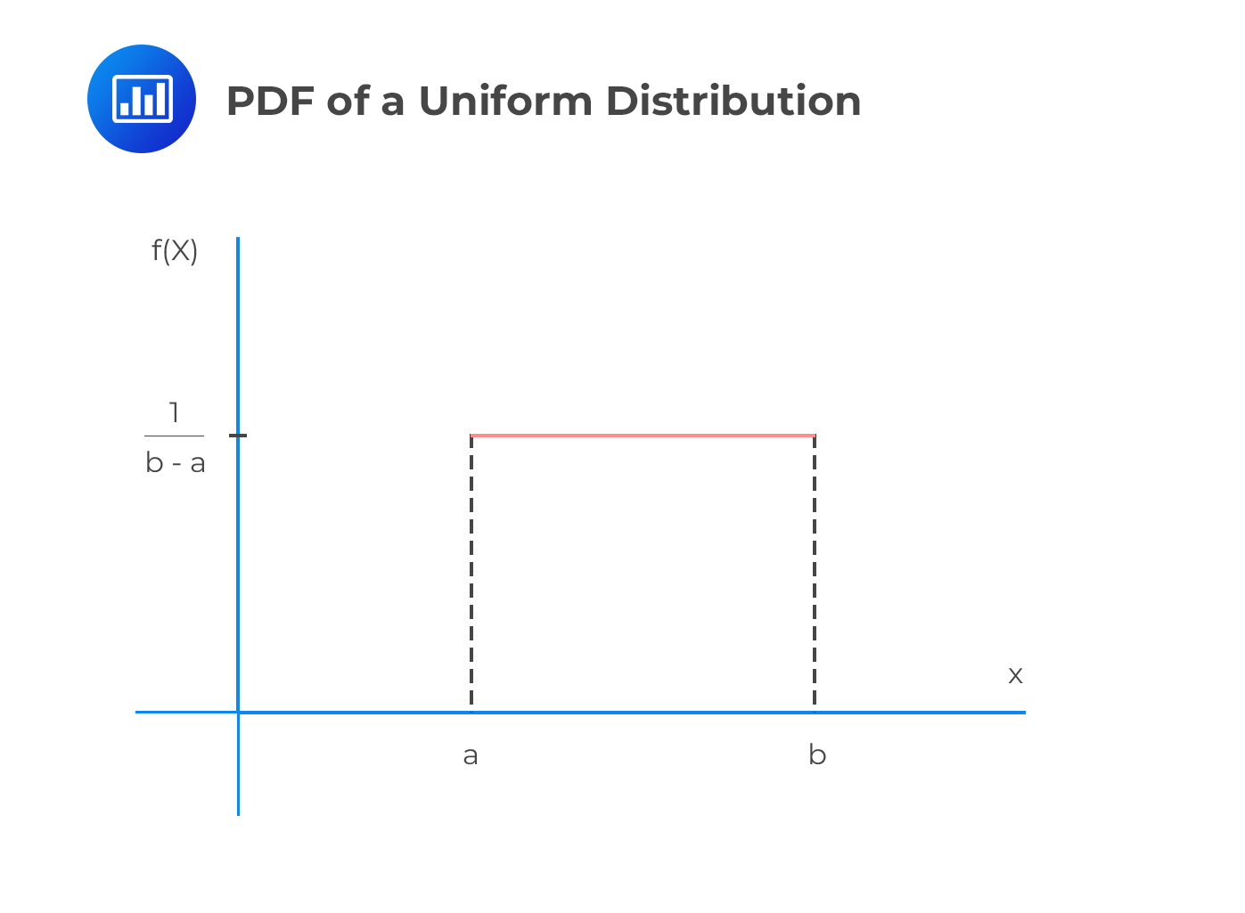 Note that the PDF of a uniform random variable does not depend on x since all values are equally likely.
The CDF of the uniform distribution is:
$$F_X(x)=\begin{cases} &0, x<a \\ &\frac{x-a}{b-a}, a≤x≤b \\ &1, x≥b \end{cases}$$
When a=0 and b=1, the distribution is called the standard uniform distribution. From this distribution, we can construct any uniform distribution, \(U_2\) and \(U_1\) using the formula:
$$U_2=a+ \left(b-a \right) U_1$$
Where a and b are limits of \(U_2\)
The uniform distribution is denoted by \(X \sim U(a,b)\), and the mean and variance are given by:
$$E(X)= \frac{a+b}{2}$$
$$V(X)=\frac{(b-a)^2}{12}$$
For instance, the variance of the standard uniform distribution \(U_1\sim N(0,1) \) is given by:
$$E(X)=\frac{(0+1)}{2}=\frac{1}{2}$$
And
$$V(X)=\frac{(1-0)^2}{12}=\frac{1}{12}$$
Assume that we want to calculate the probability that X falls in the interval \(l<X<u\) where l is the lower limit and u is the upper limit. That is, we need \(P(l<X<u)\) given that \(X \sim U(a,b)\). To compute this, we use the formula:
$$P(l<X<u)=\frac{min(u,b)-max(l,a)}{b-a}$$
Intuitively, if \(l≥a\) and \(u≤b\), the formula above simplifies into:
$$\frac{u-l}{b-a}$$
Given the uniform distribution \(X~U(-5,10)\), calculate the mean, variance, and \(P(-3<X<6)\).
Solution
For uniform distribution,
$$E(X)= \frac{a+b}{2}=\frac{-5+10}{2}=2.5$$
And
$$V(X)=\frac{(10–5)^2}{12}=\frac{225}{12}=18.75$$
For \(P(-3<X<6)\), using the formula:
$$P(l<X<u)=\frac{min(u,b)-max(l,a)}{b-a}$$
$$P(-3<X<6)=\frac{min(6,10)-max(-3,-5)}{10–5}=\frac{6–3}{10–5}=\frac{9}{15}=0.60$$
Alternatively, you can think of the probability as the area under the curve. Note that the height of the uniform distribution is \(\frac{1}{b-a}\) and the length \(u-l\).
That is:
$$\frac{1}{b-a} \times (u-l)= \frac{1}{10–5} \times (6–3)=\frac{9}{15}=0.60$$
Also called the Gaussian distribution, the normal distribution has a symmetrical PDF, and the mean and median coincide with the highest point of the PDF. Furthermore, the normal distribution always has a skewness of 0 and a kurtosis of 3.
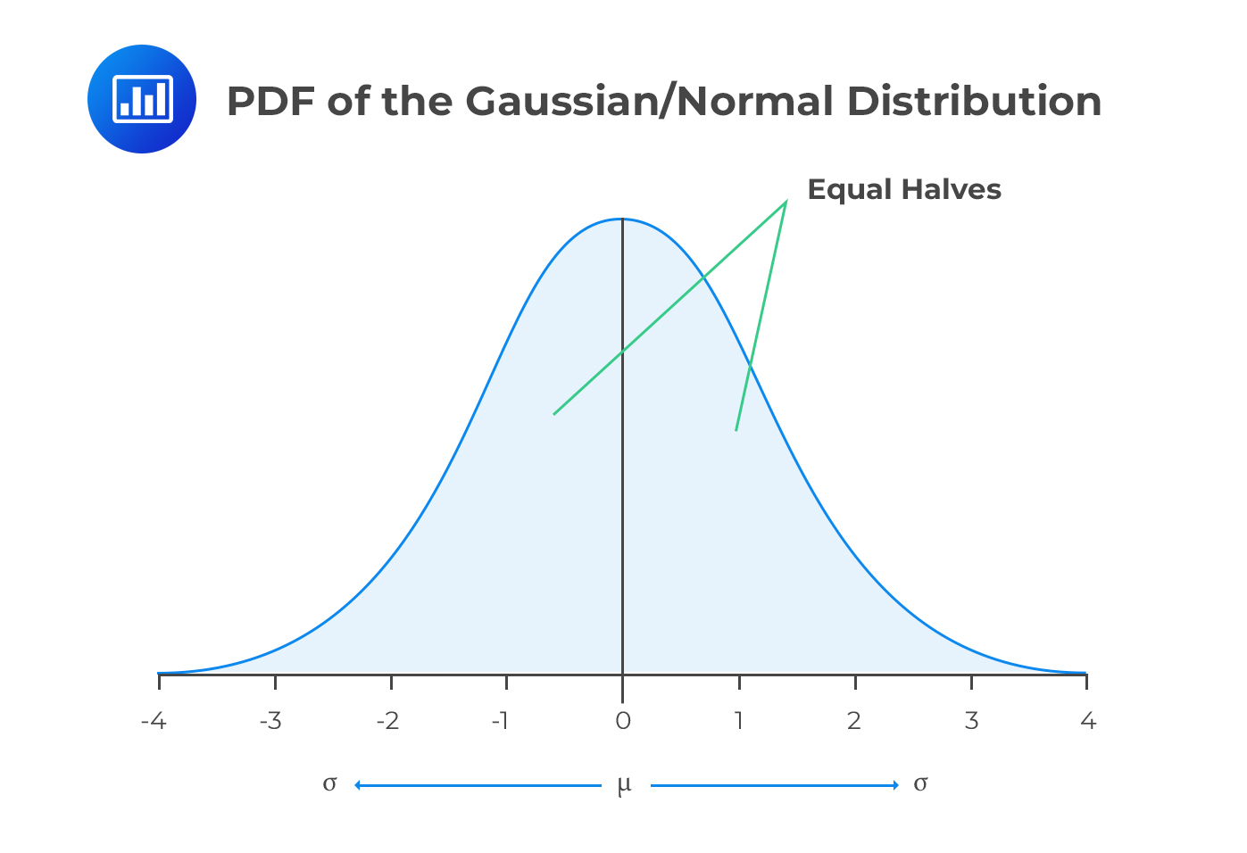 The following is the formula of a PDF that is normally distributed, for a given random variable \(X\):
$$ f\left( x \right) =\frac { 1 }{ \sigma \sqrt { 2\pi } } { e }^{ -\cfrac { 1 }{ 2 } { \left( \cfrac { x-\mu }{ \sigma } \right) }^{ 2 } }, -\infty <x< \infty $$
When a variable is normally distributed, it is often written as follows, for convenience:
$$ X\sim N\left( \mu ,{ \sigma }^{ 2 } \right) $$
Where \(E(X)= μ\) and \(V(X)= σ^2\)
We read this as \(X\) is normally distributed,with a mean, \(\mu\),and variance of \({ \sigma }^{ 2 } \). Any linear combination of independent normal variables is also normal. To illustrate this, assume \(X\) and \(Y\) are two variables that are normally distributed. We also have constants \(a\) and \(b\). Then \(Z\) will be normally distributed such that:
$$ Z=aX+bY,\quad such\quad that\quad Z\sim N\left( a{ \mu }_{ X }+b{ \mu }_{ Y },{ a }^{ 2 }{ \sigma }_{ X }^{ 2 }+{ b }^{ 2 }{ \sigma }_{ Y }^{ 2 } \right) $$
For instance for \(a=b=1\), then \(Z=X+Y\) and thus \(Z \sim N(μ_X+μ_Y,σ_X^2+σ_Y^2)\)
A standard normal distribution is a normal distribution whose mean is 0 and standard deviation is 1.It is denoted by N(0,1) and its PDF is as shown below:
$$ \emptyset =\frac { 1 }{ \sqrt { 2\pi } } { e }^{ -\frac { 1 }{ 2 } { x }^{ 2 } } $$
To determine a normal variable whose standard deviation is \(\sigma\) and mean is \(\mu\), we compute the product of the standard normal variable with \(\sigma\) and then add the mean:
$$ X=\mu +\sigma \emptyset \Rightarrow X\sim N\left( \mu ,{ \sigma }^{ 2 } \right) $$
Three standard normal variables \({ X }_{ 1 }\), \({ X }_{ 2 }\), and \({ X }_{ 3 }\) are combined in the following way to construct two normal variables that are correlated:
$$ { X }_{ A }=\sqrt { \rho } { X }_{ 1 }+\sqrt { 1-\rho } { X }_{ 2 } $$
$$ { X }_{ B }=\sqrt { \rho } { X }_{ 1 }+\sqrt { 1-\rho } { X }_{ 3 } $$
Where \({ X }_{ A }\) and \({ X }_{ B }\) have a correlation of \(\rho\), and are standard normal variables.
The z-value measures how many standard deviations the corresponding x value is above or below the mean. It is given by:
$$\Phi \left(z \right)=\frac{X-\mu}{\sigma} \sim N(0,1)$$
And
$$X \sim N(\mu {\sigma}^2)$$
Converting X normal random variables is termed as standardization. The values of z are usually tabulated.
For example, consider the normal distribution X~N(1,2). We wish to calculate P(X>2).
Solution
For
$$P(X>2)=1-P(X≤2)=1-\frac{2-1}{\sqrt{2}}=0.2929\approx 0.29$$
We look up this value from the z-table.
$$\Phi \left(0.29\right) \approx. 61.41\%$$
$$ \begin{array}{c|c} \textbf{x-value} & \textbf{z-value} \\ \hline \mu & \text{0} \\ \mu +1\sigma & \text{1} \\ \mu +2\sigma & \text{2} \\ \mu +n\sigma & \text{n} \\ \end{array} $$
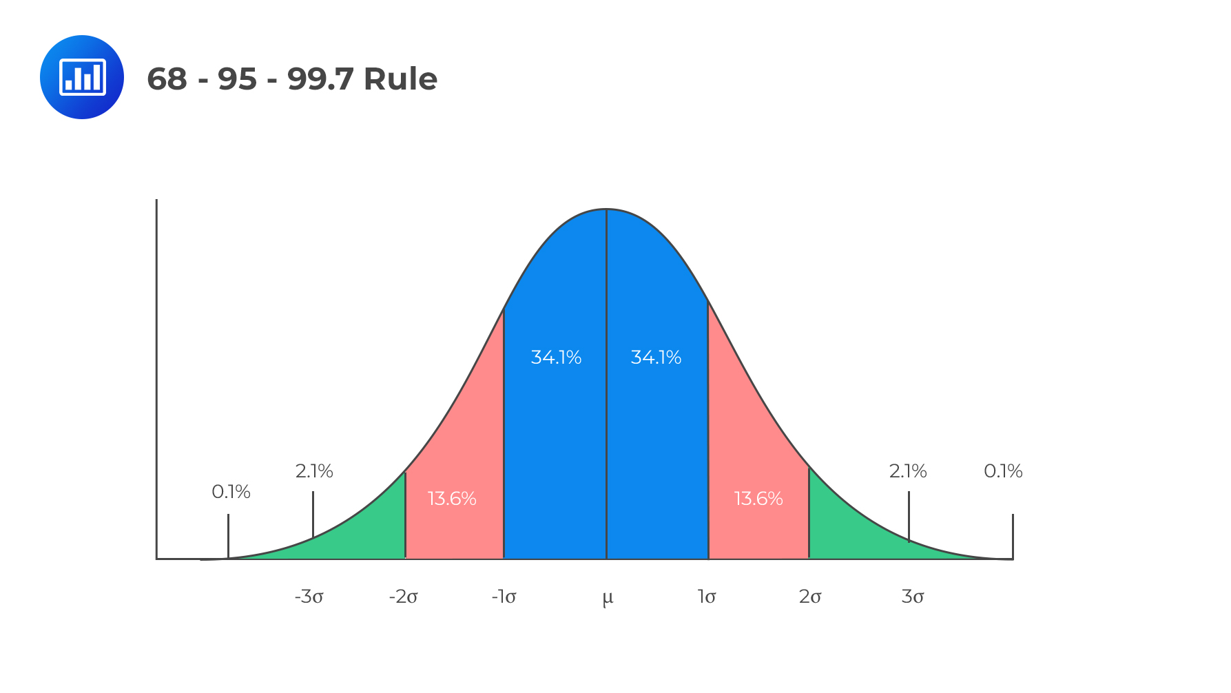 Recall that for a binomial random variable, if \(np≥10\) and \(n(1-p)≥10\), then the binomial distribution is normally distributed as:
$$X \sim N \left(np, n(1-p) \right) $$
Also, Poisson distribution is normally approximated as λ≥1000 so that:
$$X \sim N \left(λ,λ \right)$$
We then calculate the probabilities while maintaining the normal distribution principles. The normal distribution is very popular as compared to other distributions because:
A variable X is said to be lognormally distributed if the variable Y is normally distributed such that:
$$Y=lnX$$
This also can be treated as:
$$X=e^Y$$
Where
$$Y\sim N \left( \mu ,{\sigma}^2 \right)$$
Since \(Y \sim N\left(\mu, {\sigma}^2 \right)\) ,then the PDF of a log-normal random variable is:
$$ f\left( x \right) =\frac { 1 }{x\sigma \sqrt { 2\pi } } { e }^{ -\cfrac { 1 }{ 2 } { \left( \cfrac { ln(x)-\mu }{ \sigma } \right) }^{ 2 } }, x \ge 0 $$
A variable is said to have a lognormal distribution if its natural logarithm has a normal distribution. The lognormal distribution is undefined for negative values, unlike the normal distribution that has a range of values between negative infinity and positive infinity.
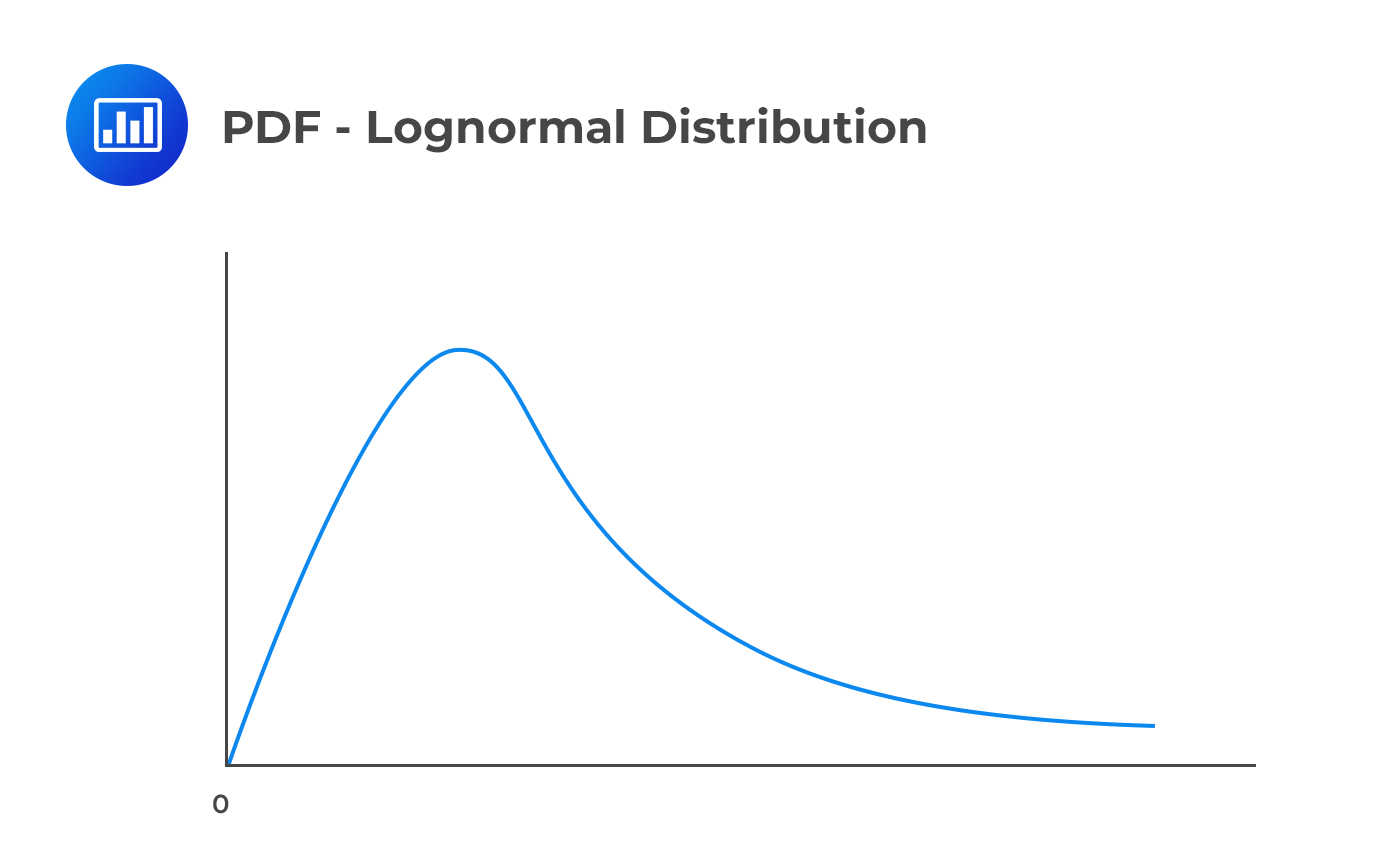 If the above equation of the density function of the lognormal distribution is rearranged, we obtain an equation that has a similar form to the normal distribution. That is:
$$ f\left( x \right) ={ e }^{ \frac { 1 }{ 2 } { \sigma }^{ 2 }-\mu }\frac { 1 }{ \sigma \sqrt { 2\pi } } { e }^{ -\frac { 1 }{ 2 } { \left( \frac { lnx-\left( \mu -{ \sigma }^{ 2 } \right) }{ \sigma } \right) }^{ 2 } } $$
From the above, we notice that the lognormal distribution happens to be asymmetrical, and not symmetrical around the mean as is the case under the normal distribution. The lognormal distribution peaks at \(exp\left( \mu -{ \sigma }^{ 2 } \right) \).
The following is the formula for the mean:
$$ E\left[ X \right] ={ e }^{ \mu +\frac { 1 }{ 2 } { \sigma }^{ 2 } } $$
This yields to an expression that closely resembles the Taylor expansion of the natural logarithm around 1. Recall that:
$$ r\approx R-\frac { 1 }{ 2 } { R }^{ 2 } $$
where \(R\) is a standard return and \(r\) is the corresponding log return.
The following is the formula for the variance of the lognormal distribution:
$$ V(X)=E\left[ \left( X-E{ \left[ X \right] }^{ 2 } \right) \right] =\left( { e }^{ { \sigma }^{ 2 } }-1 \right) { e }^{ 2\mu +{ \sigma }^{ 2 } } $$
Consider a lognormal distribution given by \(X \sim LogN(0.08,0.2)\) . Calculate the expected value.
Solution
For the lognormal distribution, the expected value is given by:
$$ E[X] ={ e }^{ \mu +\frac { 1 }{ 2 } { \sigma }^{ 2 } } ={ e }^{ 0.08 +\frac { 1 }{ 2 } { 0.2 }^{ 2 } } =1.1052 $$
Assume we’ve got k independent standard normal variables ranging from \({ Z }_{ 1 }\) to \({ Z }_{ k }\). The sum of their squares will then have a Chi-Square distribution, written as follows:
$$ S=\sum _{ 1=1 }^{ k }{ { Z }_{ i }^{ 2 } } $$
So, we can denote chi-distribution as:
$$ S\sim { X }_{ k }^{ 2 } $$
\(k\) is called the degree of freedom. It is important to note that two chi-squared variables that are independent, with degrees of freedom as \({ k }_{ 1 } \) and \({ k }_{ 2 } \), respectively, have a sum that is chi-square distributed with \( \left( { k }_{ 1 } + { k }_{ 2 } \right) \) degrees of freedom.
The chi-squared variable is usually asymmetrical and takes on non-negative values only. The distribution has a mean of \(k\) and a standard deviation of \(2k\).
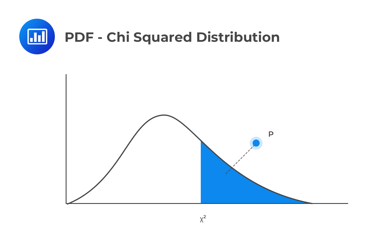 The distribution has a mean and variance given by:
$$E \left(S \right)=k$$
and
$$V \left(S \right)=2k$$
The chi-squared distribution takes the following PDF, for positive values of \(x\):
$$ f\left( x \right) =\frac { 1 }{ { 2 }^{ \frac { k }{ 2 } }\Gamma \left( \frac { k }{ 2 } \right) } { x }^{ \frac { k }{ 2 } -1 }{ e }^{ -\frac { x }{ 2 } } $$
The gamma function, \(\Gamma\), is such that:
$$ \Gamma \left( n \right) =\int _{ 0 }^{ \infty }{ { x }^{ n-1 }{ e }^{ -x }dx } $$
Note also that the gamma function,\( \Gamma \)is such that:
$$\Gamma \left(n \right)=(n-1)! $$
For instance:
$$\Gamma \left(3 \right)=(3-1)!=2 \times 1=2 $$
This distribution is widely applicable in statistics and risk management when testing hypotheses. The chi-distribution is approximated using normal distribution when n is large. This implies that:
$${\chi}^2_k \sim N \left(k,2k \right)$$
This is true because as the number of degrees of freedom increases, the skewness reduces. Degrees of freedom measures the amount of data required to test model parameters
If we have a sample size n, the degrees of freedom are given by n – p, where p is the number of parameters estimated.
This distribution is often called the \(t\) distribution.
Let Z be the standard normal variable, and U a chi-square variable with k degrees of freedom. Also, assume that U is independent of Z. Then, a random variable X that follows a t distribution is such that:
$$ X=\frac { Z }{ \sqrt { \frac { U }{ k } } } $$
The following formula represents its PDF:
$$ f\left( x \right) =\frac { \Gamma \left( k+\frac { 1 }{ 2 } \right) }{ \sqrt { k\pi } \Gamma \left( \frac { k }{ 2 } \right) } { \left( 1+{ { x }^{ 2 } }/{ k } \right) }^{ -\frac { k+1 }{ 2 } } $$
The mean of the \(t\) distribution is usually zero, and the distribution is symmetrical around it.
That is:
$$E \left(X \right)=0$$
The variance is given by:
$$V(X)=\frac{k}{k-2}$$
The kurtosis is also given by:
$$Kurt(X)=3 \frac{k-2}{k-4}$$
It is easy to see that the mean is valid for \(k>1\) and the variances finite for \(v>2\). The kurtosis is only definite if \(k>4\) and should always be higher than 3.
The distribution converges to a standard normal distribution as k tends towards infinity \((k→∞)\). When \(k>2\), the variance of the distribution becomes:\( \frac{k}{(k−2)}\), and it converges to one as \(k\) increases.
We can also separate the degrees of freedom from variance to get what we called the standardized student’s t. Using the formula:
$$V(aX)=a^2 V(X))$$
Using this result, it is easy to see that :
$$V \left[\sqrt{\frac{v-2}{v}}Y \right]=1$$
Where
$$X \sim t_k$$
The generalized student’s t is called standardized student’s t because it has a mean of 0 and a variance of 1. Note that we still rescale it to have any variance for k>2.
A generalized student’s t is stated by the mean, variance, and the number of degrees of freedom. It is stated as \(Gen.t_k (μ,σ^2) \)
This distribution is widely applicable in hypotheses testing, and modeling the returns of financial assets due to the excess kurtosis it displays.
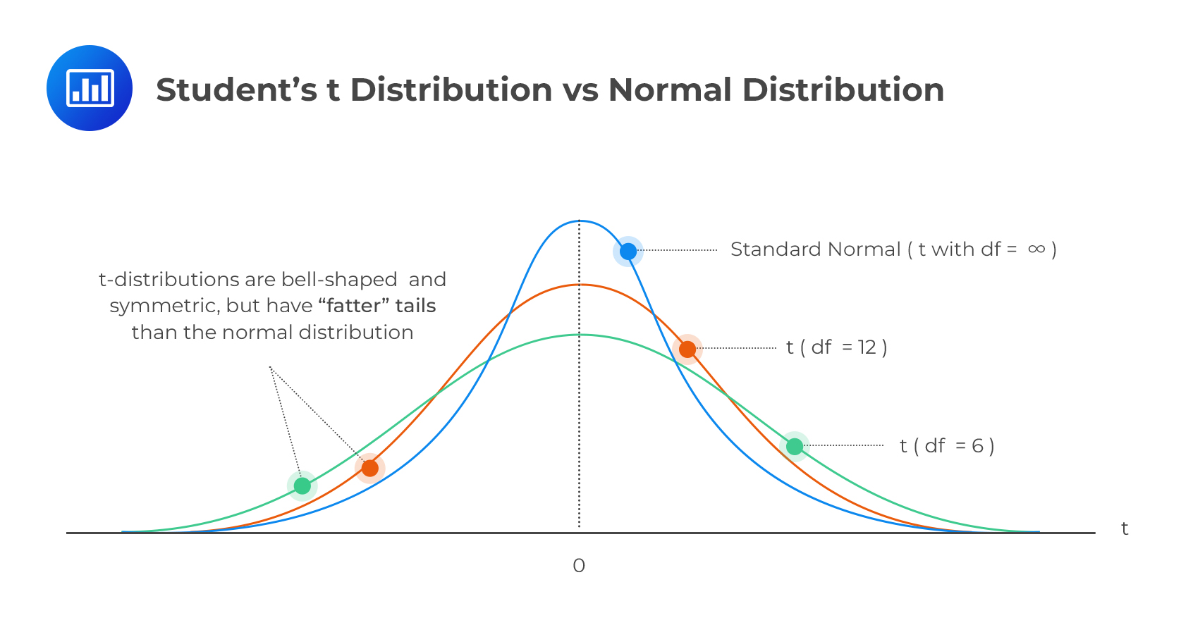 Example: Standardized Student’s t
The kurtosis of some returns on a bond portfolio with three parameters to be estimated is 6. What are degrees of freedom if the parameters were generated using student’s \(t_k\)?
Solution
We know that for t-distribution:
$$Kurt(X)=3 \frac{k-2}{k-4}$$
$$\therefore 6=3 \frac{k-2}{k-4} \Rightarrow \frac{5}{3} \left(k-4 \right)$$
So that
$$k=6$$
The F-distribution is often used in the analysis of variance (ANOVA). The F distribution is an asymmetric distribution that has a minimum value of 0, but no maximum value. Notably, the curve approaches but never quite touches the horizontal axis.
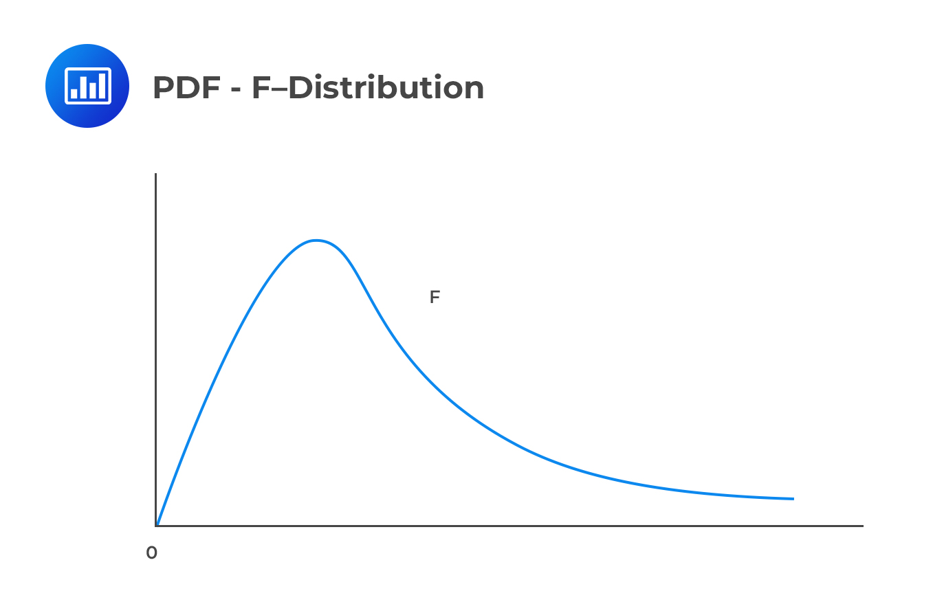 \(X\) is said to follow an \(F\)-distribution with parameters \({ k }_{ 1 }\) and \({ k }_{ 2 }\) if:
$$ X=\frac { { { U }_{ 1 } }/{ { k }_{ 1 } } }{ { { U }_{ 2 } }/{ { k }_{ 2 } } } \sim F\left( { k }_{ 1 },{ k }_{ 2 } \right) $$
Provided that \({ U }_{ 1 }\) and \({ U }_{ 2 }\) are chi-squared distributions that are independent having \({ k }_{ 1 }\) and \({ k }_{ 2 }\) as their degrees of freedom.
The \(F\)-distribution has the following PDF:
$$ f\left( x \right) =\frac { \sqrt { \frac { { \left( { k }_{ 1 }X \right) }^{ { k }_{ 1 } }{ { k } }_{ 2 }^{ { k }_{ 2 } } }{ { \left( { k }_{ 1 }X+{ k }_{ 2 } \right) }^{ { k }_{ 1 }+{ k }_{ 2 } } } } }{ xB\left( \frac { { k }_{ 1 } }{ 2 } ,\frac { { k }_{ 2 } }{ 2 } \right) } $$
B(x,y) is a beta function such that:
$$ B\left( x,y \right) =\int _{ 0 }^{ 1 }{ { z }^{ x-1 }{ \left( 1-z \right) }^{ y-1 }dz } $$
The distribution has the following mean and variance respectively:
$$ E\left(X \right) =\frac { { k }_{ 2 } }{ { k }_{ 2 }-2 } for\quad { k }_{ 2 }>2 $$
$$ { \sigma }^{ 2 }=\frac { 2{ k }_{ 2 }^{ 2 }\left( { k }_{ 1 }+{ k }_{ 2 }-2 \right) }{ { k }_{ 1 }{ \left( { k }_{ 2 }-2 \right) }^{ 2 }\left( { k }_{ 2 }-4 \right) } for\quad { k }_{ 2 }>4 $$
Suppose that \(X\) is a random variable with a \(t\)-distribution, and it has \(k\) degrees of freedom, then \({ X }^{ 2 }\) is said to have an \(F\)-distribution with 1 and \(k\) degrees of freedom, i.e.,
$$ { \chi }^{ 2 }\sim F\left( 1,k \right) $$
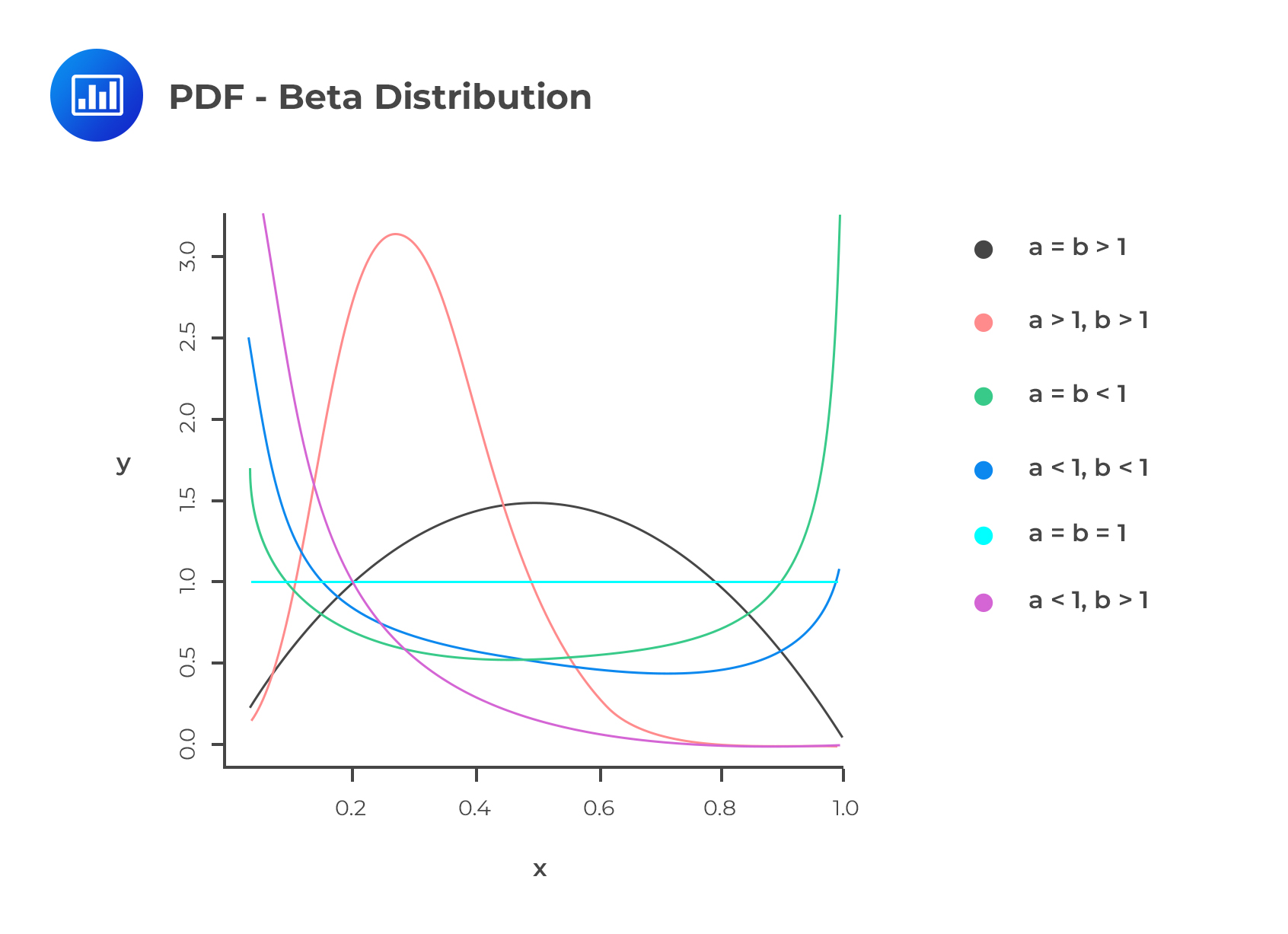
The beta distribution applies to continuous random variables in the range of 0 and 1. This distribution is similar to the triangle distribution in the sense that they are both applicable in the modelling of default rates and recovery rates. Assuming that \(a\) and \(b\) are two positive constants, then the PDF of the beta distribution is written as:
$$ f\left( x \right) =\frac { 1 }{ B\left( a,b \right) } { x }^{ a-1 }{ \left( 1-x \right) }^{ b-1 },\quad \quad \quad 0\le x\le 1 $$
Where \( B \left(a,b \right)=\frac{\Gamma (a) \Gamma (b)}{\Gamma (a+b)}\)
The following two equations represent the mean and variance of the beta distribution:
$$ \mu =\frac { a }{ a+b } $$
$$ { \sigma }^{ 2 }=\frac { ab }{ { \left( a+b \right) }^{ 2 }\left( a+b+1 \right) } $$
 Exponential Distribution
The exponential distribution is a continuous distribution with a parameter , whose PDF is:
$$ f_X(x)=\frac{1}{\beta} e^{-\frac{x}{\beta}}, x≥0$$
The CDF is also given by:
$$F_X(x)=1-e^{-\frac{x}{\beta}}$$
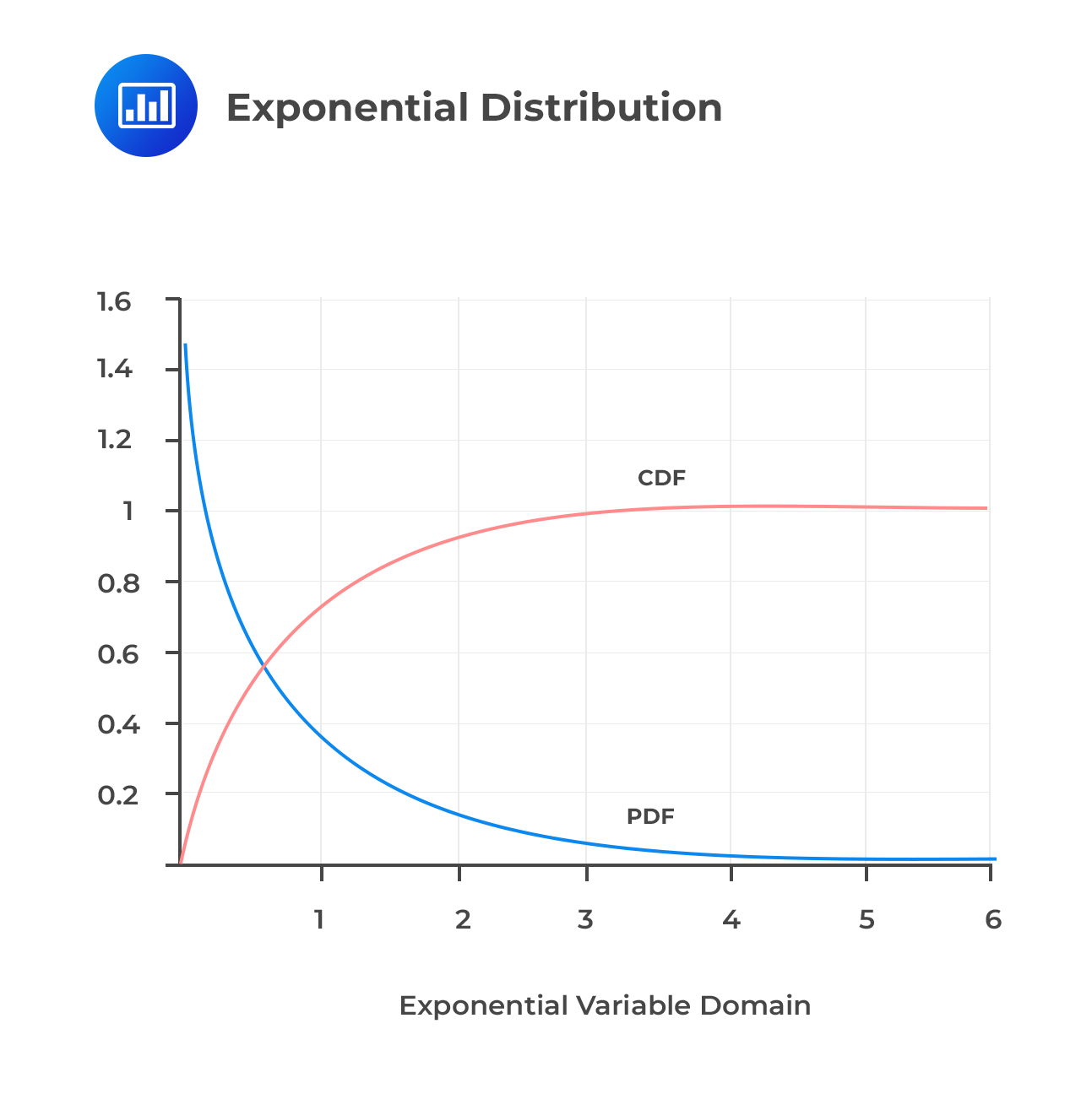 The parameter of the exponential distribution determines the mean and variance of the distribution. That is:
$$E(X)=\beta$$
And
$$V(X)={\beta}^2$$
Notably, exponential distribution is a close ‘cousins’ of a Poisson. The time intervals between one and subsequent Poisson random variables are exponentially distributed. Another feature of the exponential distribution is that it is memoryless. That is, its distributions are independent of their histories.
Assume that the time to default for a specific segment of mortgage consumers is exponentially distributed with a \(\beta\) of ten years. What is the probability that a borrower will not default before year 11?
Solution
To find the probability that the borrower will not default before year eleven, we start by calculating the cumulative distribution until year eleven and then subtract this from 100%::
$$P(X>11)=1-P(X≤11)=1-F_X (x=11)$$
$$=1-e^{-\frac{11}{10}}=1-0.3329=0.6671=66.7\%$$
Mixture distributions are complex, and new distributions built using two or more distributions. In this summary, we shall concentrate on the two distributions.
Generally, a mixture distribution comes from a weighted average distribution of density functions, and can be written as follows:
$$ f\left( x \right) =\sum _{ j=1 }^{ n }{ { w }_{ i }{ f }_{ i }\left( x \right) } \quad such\quad that:\sum _{ i=1 }^{ n }{ { w }_{ i }=1 } $$
\({ f }_{ i }\left( x \right) \)’s are the component distributions, with \({ w }_{ i }^{ \prime }\)s as the weights or the mixing proportions. The component weights must all sum up to one, for the resulting mixture to be legitimately distributed.In other words, a two-distribution combination must draw value from Bernoulli random variables and depending on the benefits (0 or 1), it then picks the component distributions. By doing this, it is possible to compute the CDF of the mixture when the component distributions are normal random variables. These distributions are very flexible as they fall between parametric and non-parametric distributions.
For example, consider \(X_1 \sim F_{x_1}\) and \(X_2 \sim F_{x_2}\) and \(W_i \sim Bernoulli (p) \) . So that the mixture distribution of \(X_1\) and \(X_2\) is given by:
$$Y=pX_1+(1-p) X_2$$
Both of the PDF and the CDF of the mixture distribution are weighted average of the constituent CDFs and PDFs. That is:
$$F_Y(y)=pF_{X_1 } (x_1 )+(1-p)F_{X_2 } (x_2 )$$
And
$$f_Y(y)=pf_{X_1 } (x_1 )+(1-p)f_{X_2 } (x_2 )$$
Intuitively, the computation of the central moment is done in a similar way. That is:
$$E(Y)= pE(X_1 )+(1- p)E(X_2)$$
And
$$V(Y)=E(Y^2 )-(E(Y))^2$$
Where
$$ E(Y^2 )=pE(X_1^2 )+(1- p)E(X_2^2) $$
Using the same logic, we can calculate the other higher central moments such as the kurtosis and skewness. However, note that the mixture distribution might have both the skewness and the kurtosis, while the components do not have (for example, normal random variables).
Moreover, mixing components with different means and variances leads to distribution that is both skewed and heavy-tailed.
Consider two normal random variables \(X_1 \sim N(0.15, 0.60)\) and \(X_1 \sim N(-0.8, 3)\). . What is the mean of the resulting mixture distribution (Y) if the weight of \(X_1\) is 0.6?
Solution
We know that:
$$\begin{align*}E(Y)&= pE(X_1 )+(1- p)E(X_2)\\&= 0.6×0.15+(1- 0.6)(-0.8)\\&=-0.23\end{align*}$$
Question
The number of new clients that a wealth management company receives in a month is distributed as a Poisson random variable with mean 2. Calculate the probability that the company receives exactly 28 clients in a year.
A. 5.48%
B. 0.10%
C. 3.54%
D. 10.2%
The correct answer is A.
The number of clients in a year (2 × 12) has a Poi(24) distribution.
$$ P\left[ X=n \right] =\frac { { \lambda }^{ n } }{ n! } { e }^{ -\lambda } $$
$$ P\left[ X=28 \right] =\frac { { 24 }^{ 28 } }{ 28! } { e }^{ -24 }=5.48% $$
Get Ahead on Your Study Prep This Cyber Monday! Save 35% on all CFA® and FRM® Unlimited Packages. Use code CYBERMONDAY at checkout. Offer ends Dec 1st.