Properties of Continuous Uniform Distr ...
The continuous uniform distribution is such that the random variable \(X\) takes values... Read More
The probability distribution of a random variable “X” is basically a graphical presentation of the probabilities of all possible outcomes of X. A random variable is any quantity for which more than one value is possible. An example of a random variable is the price of quoted stocks. Simply put, a probability distribution gathers all the outcomes and goes a step further to indicate the probability associated with each outcome.
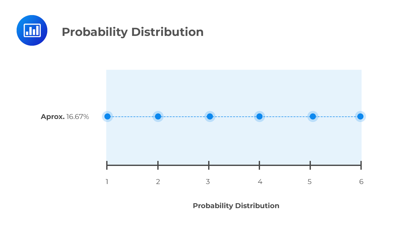
Practice probability distributions and random variable questions with CFA®-style problems.{1 2 3 4 5 6}
Each of these outcomes would occur with a probability of 1/6 because each of them has an equal chance of occurring. Consequently, the probability distribution would be a straight line:

Note to candidates: although the above distribution is a straight line, most real life distributions are usually curved. The CFA curriculum particularly delves into the bell-shaped normal distribution.
A discrete random variable can take on a finite number of outcomes.
Examples
A continuous random variable is that which has an infinite number of possible outcomes. A good example can be the rate of return on a stock. For instance, the return can be 6% or between 6% and 7%, in which case it can take on 6.4%, 6.41%, 6.412%, or even 6.412325%, i.e., infinite values.
A probability function gives the probability of a random variable X taking on a value “x.” The probability functions of discrete and continuous random variables are slightly different.
For a discrete random variable, the probability function, P(x), satisfies the properties below.
For a continuous random variable, the probability function, f(x), satisfies the properties listed below.
Reading 9 LOS 9a:
Define a probability distribution and distinguish between discrete and continuous random variables and their probability functions.
Get Ahead on Your Study Prep This Cyber Monday! Save 35% on all CFA® and FRM® Unlimited Packages. Use code CYBERMONDAY at checkout. Offer ends Dec 1st.