Using a Timeline to Model Cash Flows and Solve Time Value of Money Problems

A timeline is a physical illustration of the amounts and timing of cash flows associated with an investment project. Cash flows that are regular and of equal amounts can be modeled as annuities. In such exam problems, all you have to do is apply the standard annuity formulas. It is even more convenient if you use the approved calculators to do most of the work. However, it may get a little tricky if the cash flows are irregular, unequal, or both. It is essential to draw a timeline to help you understand the problem.

Remember that the general formula that relates the present value and the future value of an investment is given by:

$$FV_{N}=PV\left(1+r\right)^{N}$$

Where

PV = present value of the investment
FV_N = future value of the investment N periods from today
r = rate of interest per period

We can represent this in a timeline:

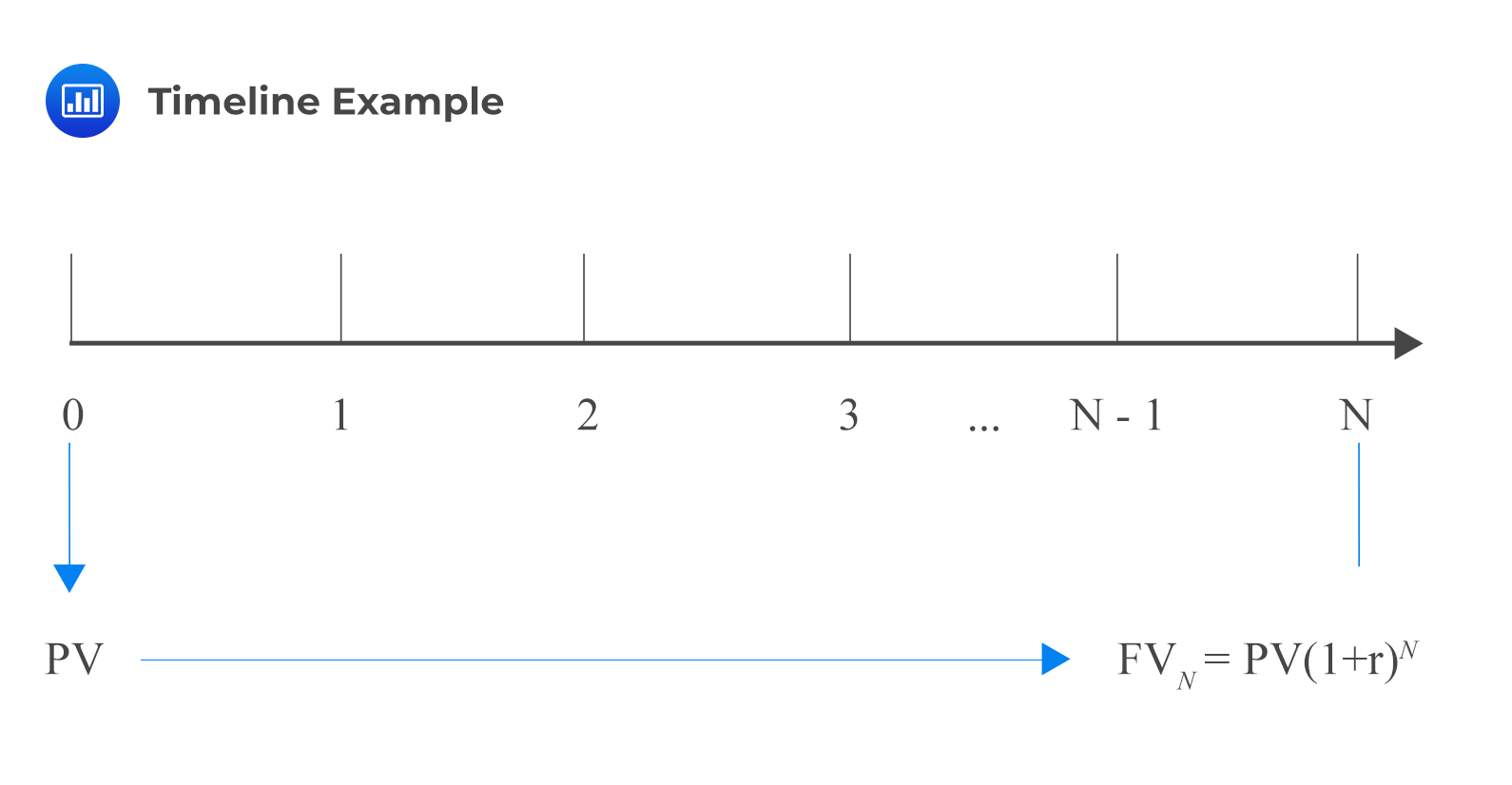
A timeline visualizes the compatibility between the time units and the corresponding interest rate per unit time. In a particular timeline, a time index t represents a particular point in time, a specified number of periods from today. Therefore, the present value is the investment amount today (t=0). We can use this amount to calculate the future value (t=N). Alternatively, we can use the future value to calculate the present value.

The above argument can be written in terms of the present value. That is:

$$PV=FV_{N}\left(1+r\right)^{-N}$$

Example: Applying Timeline to Model Cashflows

An investor receives a series of payments, each amounting to $6,500, set to be received in perpetuity. Payments are to be made at the end of each year, starting at the end of year 4. If the discount rate is 9%, then what is the present value of the perpetuity at t=0?

Solution

We should draw a timeline to understand the problem better.

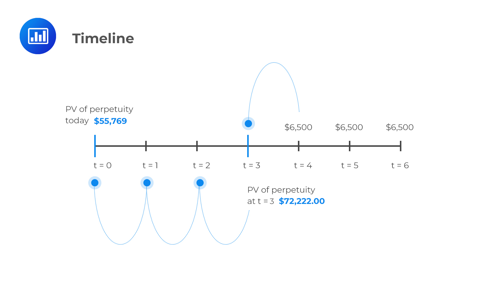
Here, we can see that the investor is receiving $6,500 in perpetuity (lasts forever). Note that the PV of a PV is given by:

$$\text{PV of a perpetuity} =\frac {C}{r}$$

So that in this case:

$$\text{PV}=\frac {$6,500}{9\%} = $72,222$$

This is the value of the perpetuity at t=3, so we need to discount it 3 more periods to get the value at t=0. Here is the formula to use:

$$PV=FV_{N}\left(1+r\right)^{-N}$$

PV at time zero =\( \frac {$72,222}{{(1+0.09)}^3} = $55,769\)

Why is the Use of a Timeline Recommended?

There are many instances in real life when cash flows are uneven. A good case in point is pension contributions which vary with age. In such problems, it’s not possible to apply one of the basic time value formulae. You’re advised to draw a timeline even if the question appears quite straightforward. The timeline will help you understand the question structure better. A timeline also helps candidates add cash flows indexed to the same period and apply the value additivity principle.

Question

Assume that we have two projects, X and Y, and each has positive cash flows. The annual interest rate is 5% per year. The projects have the following cash flows;

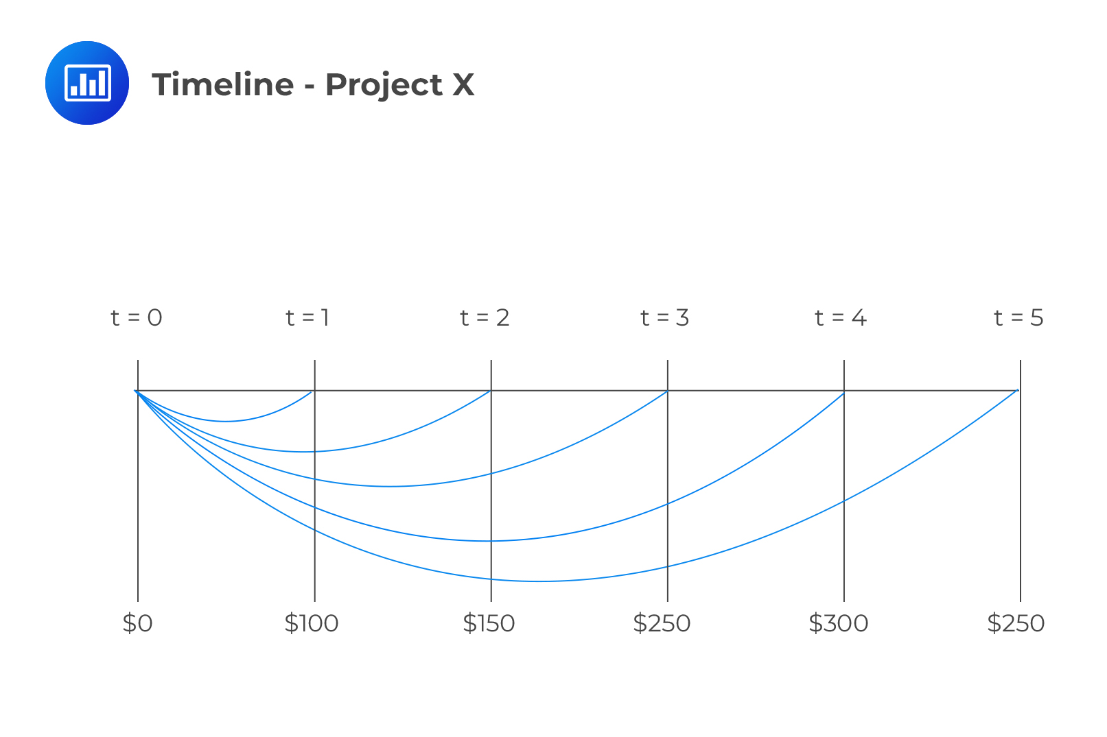
X: $100 at t = 1, $150 at t = 2, $250 at t = 3, $300 at t = 4 and $250 at t = 5

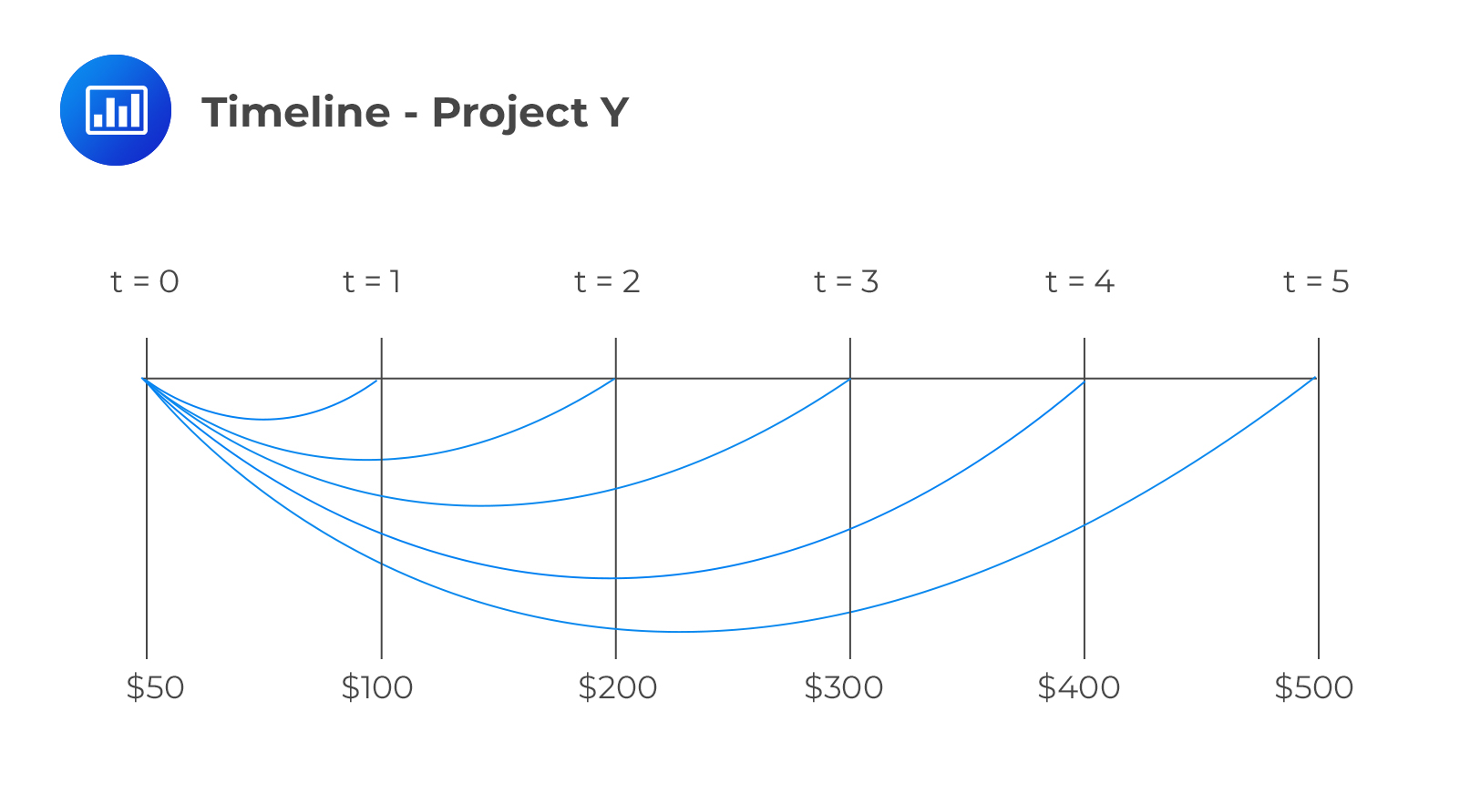
Y: $50 at t = 0, $100 at t = 1, $200 at t = 2, $300 at t = 3, $400 at t = 4 and $500 at t = 5 where t = time in years

Project X:

$$ \begin{array}{c|c|c|c|c|c} {t=0} & {t=1} & {t=2} & {t=3} & {t=4} & {t=5} \\ \hline {$0 } & {$100 } & {$150 } & {$250 } & {$300 } & {$250 } \\ \end{array} $$

Project Y:

$$ \begin{array}{c|c|c|c|c|c} {t=0} & {t=1} & {t=2} & {t=3} & {t=4} & {t=5} \\ \hline {$50 } & {$100 } & {$200 } & {$300 } & {$400 } & {$500 } \\ \end{array} $$

What is the present value of the cash flows for both projects combined?

A. $890

B. $2,197

C. $1,307

Solution

The correct answer is B.

The time project X is as follows:

We can calculate the cash flows for each project and then add them up.

$$ \begin{align*}
\text{PV for X} & = 100(1 + r)^{-1} + 150(1 + r)^{-2} + 250(1 + r)^{-3} + 300(1 + r)^{-4} + 250(1 + r)^{-5} \\
& = 100 \times 1.05^{-1} + 150 \times 1.05^{-2} + 250 \times 1.05^{-3} + 300 \times 1.05^{-4} + 250 \times 1.05^{-5} \\
& = $890\end{align*} $$

For project Y, the timeline is given by:

$$ \begin{align*} \text{PV for Y} & = 50(1 + r)^{-0}+ 100(1 + r)^{-1} + 200(1 + r)^{-2} + 300(1 + r)^{-3} + 400(1 + r)^{-4} + 500(1 + r)^{-5} \\
& = 50 + 100 \times 1.05^{-1} + 200 \times 1.05^{-2} + 300 \times 1.05^{-3} + 400 \times 1.05^{-4} + 500 \times1.05^{-5} \\
& = $1307 \end{align*} $$

Hence, the net present value is = 890+1307=$2,197.

Alternatively, we can combine corresponding cash flows and work out the present values for the two projects at once i.e.

$$ \begin{array}{c} \text{NPV} = (0+50) +(100+100) \times 1.05^{-1} + (150+200)\times 1.05^{-2}+ (250+300) \times 1.05^{-3} + \\ (300+400) \times 1.05^{-4} + (250+500) \times 1.05^{-5} \\ = $2197 \\ \end{array} $$

The latter method applies the value additivity principle, which asserts that the NPV of a set of independent projects is just the sum of the NPVs of the individual projects.

We can apply this principle to find the NPVs of projects with uneven cash flows.

Reading 6 LOS 6f

Demonstrate the use of a time line in modeling and solving time value of money problems.