Measures of Fit and Hypothesis Tests of Regression Coefficients

The sum of Squares Total (SST) and Its Components

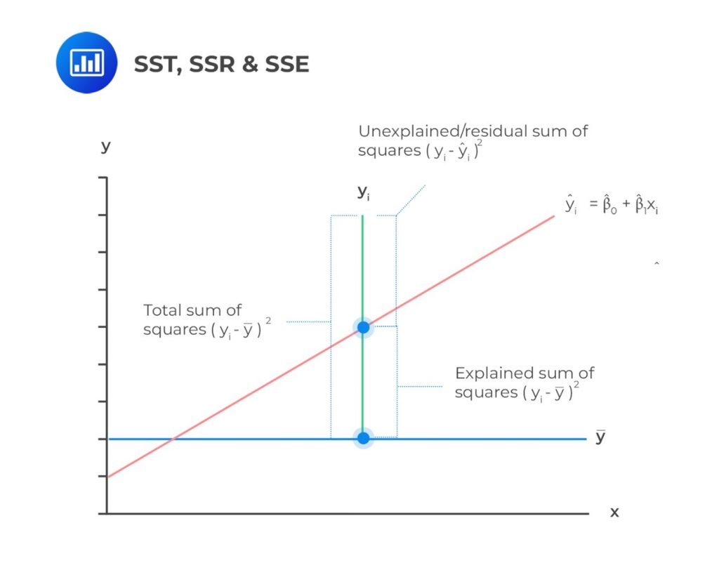
The sum of Squares Total (total variation) is a measure of the total variation of the dependent variable. It is the sum of the squared differences of the actual y-value and mean of y-observations.

$$ SST=\sum_{i=1}^{n}\left(Y_i-\bar{Y}\right)^2 $$

The Sum of Squares Total contains two parts:

1. The Sum of Square Regression (SSR).
2. The sum of Squares Error (SSE).

1. The sum of Squares Regression (SSR): The sum of squares regression measures the explained variation in the dependent variable. It is given by the sum of the squared differences of the predicted y-value \({\hat{Y}}_i\), and mean of y-observations, \(\bar{Y}\):$$ SSR=\sum_{i=1}^{n}\left({\hat{Y}}_i-\bar{Y}\right)^2 $$
2. The Sum of Squared Errors (SSE): The sum of squared errors is also called the residual sum of squares. It is defined as the variation of the dependent variable unexplained by the independent variable. SSE is given by the sum of the squared differences of the actual y-value \((Y_i)\) and the predicted y-values, \({\hat{Y}}_i\).$$ {SSE}=\sum_{i=1}^{n}\left(Y_i-{\hat{Y}}_i\right)^2 $$Therefore, the sum of squares total is given by:$$ \begin{align*} \text{Sum of Squares Total} & ={\text{Explained Variation} + \text{Unexplained Variation}} \\ & ={SSR+ SSE} \end{align*} $$

The components of the total variation are shown in the following figure.

For example, consider the following table. We wish to use linear regression analysis to forecast inflation, given unemployment data from 2011 to 2020.

$$ \begin{array}{c|c|c}
\text{Year} & {\text{Unemployment Rate } (\%)} & {\text{Inflation Rate } (\%)} \\ \hline
2011 & 6.1 & 1.7 \\ \hline
2012 & 7.4 & 1.2 \\ \hline
2013 & 6.2 & 1.3 \\ \hline
2014 & 6.2 & 1.3 \\ \hline
2015 & 5.7 & 1.4 \\ \hline
2016 & 5.0 & 1.8 \\ \hline
2017 & 4.2 & 3.3 \\ \hline
2018 & 4.2 & 3.1 \\ \hline
2019 & 4.0 & 4.7 \\ \hline
2020 & 3.9 & 3.6
\end{array} $$

Remember that we had estimated the regression line to be \(\hat{Y}=7.112-0.9020X_i+\varepsilon_i\). As such, we can create the following table:

$$ \begin{array}{c|c|c|c|c|c|c|c}
\text{Year} & \text{Unemployment} & \text{Inflation} & \text{Predicted} & \text{Variation} & \text{Variation} & \text{Variation} & (X_i \\
& {\text{Rate } \% (X_i)} & {\text{Rate }\%} & \text{Unemployment} & \text{to be} & \text{Unexplained} & \text{Explained} & -\bar{X})^2 \\
& & ({{Y}}_i) & {\text{rate } (\hat Y_i)} & \text{Explained.} & & & \\
& & & & \left(Y_i-\bar{Y}\right)^2 & \left(Y_i- \hat{Y}_i\right)^2 & \left({\hat{Y}}_i-\bar{Y}\right)^2 & \\ \hline
2011 & 6.1 & 1.7 & 1.610 & 0.410 & 0.008 & 0.533 & 0.656 \\ \hline
2012 & 7.4 & 1.2 & 0.437 & 1.300 & 0.582 & 3.621 & 4.452 \\ \hline
2013 & 6.2 & 1.3 & 1.520 & 1.082 & 0.048 & 0.673 & 0.828 \\ \hline
2014 & 6.2 & 1.3 & 1.520 & 1.082 & 0.048 & 0.673 & 0.828 \\ \hline
2015 & 5.7 & 1.4 & 1.971 & 0.884 & 0.326 & 0.136 & 0.168 \\ \hline
2016 & 5.0 & 1.8 & 2.602 & 0.292 & 0.643 & 0.069 & 0.084 \\ \hline
2017 & 4.2 & 3.3 & 3.324 & 0.922 & 0.001 & 0.967 & 1.188 \\ \hline
2018 & 4.2 & 3.1 & 3.324 & 0.578 & 0.050 & 0.967 & 1.188 \\ \hline
2019 & 4.0 & 4.7 & 3.504 & 5.570 & 1.430 & 1.355 & 1.664 \\ \hline
2020 & 3.9 & 3.6 & 3.594 & 1.588 & 0.000 & 1.573 & 1.932 \\ \hline
\textbf{Sum} & \bf{52.90} & \bf{23.4} & & \bf{13.704} & \bf{3.136} & \bf{10.568} & \bf{12.989} \\ \hline
\textbf{Arithmetic} & \bf{5.29} & \bf{2.34} & & & & & \\
\textbf{Mean} & & & & & & & \\
\end{array} $$

From the table above, we can calculate the following:

$$ \begin{align*}
SST & =\sum_{i=1}^{n}{\left(Y_i-\bar{Y}\right)^2=13.704} \\
SSR & =\sum_{i=1}^{n}\left({\hat{Y}}_i-\bar{Y}\right)^2 =10.568 \\
{SSE} & =\sum_{i=1}^{n}\left(Y_i-{\hat{Y}}_i\right)^2=3.136
\end{align*} $$

Measures of Goodness of Fit

We use the following measures to analyze the goodness of fit of simple linear regression:

1. Coefficient of determination.
2. F-statistic for the test of fit.
3. Standard error of the regression.

Coefficient of Determination

The coefficient of determination \((R^2)\) measures the proportion of the total variability of the dependent variable explained by the independent variable. It is calculated using the formula below:

$$ \begin{align*} R^2 =\frac{\text{Explained Variation} }{\text{Total Variation}}& =\frac{\text{Sum of Squares Regression (SSR)} }{\text{Sum of Squares Total (SST)}} \\ & =\frac{\sum_{i=1}^{n}\left({\hat{Y}}_i-\bar{Y}\right)^2}{\sum_{i=1}^{n}\left(Y_i-\bar{Y}\right)^2} \end{align*} $$

Intuitively, we can think of the above formula as:

$$ \begin{align*}
R^2 & =\frac{\text{Total Variation}-\text{Unexplained Variation} }{\text{Total Variation}}\\
& =\frac{\text{Sum of Squares Total (SST)}-\text{Sum of Squared Errors (SSE)} }{\text{Sum of Squares Total}} \end{align*} $$

Simplifying the above formula gives:

$$ R^2=1-\frac{\text{Sum of Squared Errors (SSE)} }{\text{Sum of Squares Total (SST)}} $$

In the above example, the coefficient of variation is:

$$ \begin{align*}
R^2 & =\frac{\text{Explained Variation} }{\text{Total Variation}} \\ & =\frac{\text{Sum of Squares Regression (SSR)} }{\text{Sum of Squares Total (SST)}} \\ & =\frac{2.973}{12.989}=22.89\% \end{align*} $$

Features of Coefficient of Determination (\(R^2\))

\(R^2\) lies between 0% and 100%. A high \(R^2\) explains variability better than a low \(R^2\). If \(R^2\)=1%, only 1% of the total variability can be explained. On the other hand, if \(R^2\)=90%, over 90% of the total variability can be explained. In a nutshell, the higher the \(R^2\), the higher the model’s explanatory power.

For simple linear regression \((R^2)\) is calculated by squaring the correlation coefficient between the dependent and the independent variables:

$$ r^2=R^2=\left(\frac{Cov\left(X,Y\right)}{\sigma_X\sigma_Y}\right)^2=\frac{\sum_{i=1}^{n}\left({\hat{Y}}_i-\bar{Y}\right)^2}{\sum_{i=1}^{n}\left(Y_i-\bar{Y}\right)^2} $$

Where:

\((Cov \left(X,Y\right))\) = Covariance between two variables, \(X\) and \(Y\).

\((\sigma_X)\) = Standard deviation of \(X\).

\((\sigma_Y)\) = Standard deviation of \(Y\).

Example: Calculating Coefficient of Determination \(({R}^{2})\)

An analyst determines that \((\sum_{i= 1}^{6}{\left(Y_i-\bar{Y}\right)^2= 13.704)}\) and \((\sum_{i = 1}^{6}\left(Y_i-{\hat{Y}}_i\right)^2=3.136)\) from the regression analysis of inflation rates on unemployment rates. The coefficient of determination \(\left((R^2)\right)\) is closest to:

Solution

$$ \begin{align*}
R^2 & =\frac{{\text{Sum of Squares Total (SST)}-\text{Sum of Squared Errors (SSE)} } }{\text{Sum of Squares Total (SST)}} \\ & =\frac{\left(\sum_{i=1}^{n}\left(Y_i-\bar{Y}\right)^2-\sum_{i=1}^{n}\left(Y_i-\hat{Y}\right)^2\right)}{\sum_{i=1}^{n}\left(Y_i-\bar{Y}\right)^2}=\frac{13.704-3.136}{13.704} \\ & =0.7712=77.12\% \end{align*} $$

F-statistic in Simple Regression Model

Note that the coefficient of variation discussed above is just a descriptive value. To check the statistical significance of a regression model, we use the F-test. The F-test requires us to calculate the F-statistic.

In simple linear regression, the F-test confirms whether the slope (denoted by \((b_1)\)) in a regression model is equal to zero. In a typical simple linear regression hypothesis, the null hypothesis is formulated as: \((H_0:b_1=0)\) against the alternative hypothesis \((H_1:b_1\neq0)\). The null hypothesis is rejected if the confidence interval at the desired significance level excludes zero.

The Sum of Squares Regression (SSR) and Sum of Squares Error (SSE) are employed to calculate the F-statistic. In the calculation, the Sum of Squares Regression (SSR) and Sum of Squares Error (SSE) are adjusted for the degrees of freedom.

The Sum of Squares Regression(SSR) is divided by the number of independent variables (k) to get the Mean Square Regression (MSR). That is:

$$ MSR=\frac{SSR}{k} = \frac{\sum_{i = 1}^{n}\left(\widehat{Y_i}-\bar{Y}\right)^2}{k} $$

Since we only have \((k=1)\), in a simple linear regression model, the above formula changes to:

$$ MSR=\frac{SSR}{1}=\frac{\sum_{i = 1}^{n}\left(\widehat{Y_i}-\bar{Y}\right)^2}{1}=\sum_{i = 1}^{n}\left({\hat{Y}}_i-\bar{Y}\right)^2 $$

Therefore, in the Simple Linear Regression Model, MSR = SSR.

Also, the Sum of Squares Error (SSE) is divided by degrees of freedom given by \((n-k-1)\) (this translates to \((n-2)\) for simple linear regression) to arrive at Mean Square Error (MSE). That is,

$$
MSE=\frac{\text{Sum of Squares Error (SSE)}}{n-k-1}=\frac{\sum_{i=1}^{n}\left(Y_i-\hat{Y}\right)^2}{n-k-1} $$

For a simple linear regression model,

$$ MSE =\frac{\text{Sum of Squares Error(SSE)}}{n-2} =\frac{\sum_{i =1 }^{n}\left(Y_i-\hat{Y}\right)^2}{n-2} $$

Finally, to calculate the F-statistic for the linear regression, we find the ratio of MSR to MSE. That is,

$$ \begin{align*} F-\text{statistic} = \frac{MSR}{MSE} = \frac{\frac{SSR}{k}}{\frac{SSE}{n-k-1}} = \frac{\frac{\sum_{i=1}^{n}\left(\widehat{Y_i}-\bar{Y}\right)^2}{k}}{\frac{\sum_{i = 1 }^{n}\left(Y_i-\hat{Y}\right)^2}{n-k-1}} \end{align*} $$

For simple linear regression, this translates to:

$$ \begin{align*} F-\text{statistic}=\frac{MSR}{MSE} =\frac{\frac{SSR}{k}}{\frac{SSE}{n-k-1}} = \frac{\sum_{i = 1}^{n}\left(\widehat{Y_i}-\bar{Y}\right)^2}{\frac{\sum_{i = 1}^{n}\left(Y_i-\hat{Y}\right)^2}{n-2}} \end{align*} $$

The F-statistic in simple linear regression is F-distributed with \((1)\) and \((n-2)\) degrees of freedom. That is,

$$ \frac{MSR}{MSE}\sim F_{1,n-2} $$

Note that the F-test regression analysis is a one-side test, with the rejection region on the right side. This is due to the fact that the objective is to test whether the variation in Y explained (the numerator) is larger than the variation in Y unexplained (the denominator).

Interpretation of F-test Statistic

A large F-statistic value proves that the regression model effectively explains the variation in the dependent variable and vice versa. On the contrary, an F-statistic of 0 indicates that the independent variable does not explain the variation in the dependent variable.

We reject the null hypothesis if the calculated value of the F-statistic is greater than the critical F-value.

It is worth mentioning that F-statistics are not commonly used in regressions with one independent variable. This is because the F-statistic is equal to the square of the t-statistic for the slope coefficient, which implies the same thing as the t-test.

Standard Error of Estimate

Standard Error of Estimate, \(S_e\) or SEE, is alternatively referred to as the root mean square error or standard error of the regression. It measures the distance between the observed dependent variables and the dependent variables the regression model predicts. It is calculated as follows:

$$ {\text{Standard Error of Estimate}}\left(S_e\right)=\sqrt{MSE}=\sqrt{\frac{\sum_{i = 1}^{n}\left(Y_i-{\hat{Y}}_i\right)^2}{n-2}} $$

The standard error of estimate, coefficient of determination, and F-statistic are the measures that can be used to gauge the goodness of fit of a regression model. In other words, these measures tell the extent to which a regression model syncs with data.

The smaller the Standard Error of Estimate is, the better the fit of the regression line. However, the Standard Error of Estimate does not tell us how well the independent variable explains the variation in the dependent variable.

Hypothesis Tests of Regression Coefficients

Hypothesis Test on the Slope Coefficient

Note that the F-statistic discussed above is used to test whether the slope coefficient is significantly different from 0. However, we may also wish to test whether the population slope differs from a specific value or is positive. To accomplish this, we use the t-distributed test.

The process of performing the t-distributed test is as follows:

1. State the hypothesis: For instance, typical hypothesis statements include:
   • \(H_0: b_1 =0 \text{ versus } H_a: b_1 \neq 0\)
   • \(H_0: b_1\le 0 \text{ versus } H_a: b_1> 0\)
2. Identify the appropriate test statistic: The test statistic for the t-distributed test on slope coefficient is given by: $$ t=\frac{{\hat{b}}_1-B_1}{s_{{\hat{b}}_1}} $$Where:\(B_1\) = Hypothesized slope coefficient.\(\widehat{b_1}\) = Point estimate for \(b_1\)\(s_{{\hat{b}}_1 }\) = Standard error of the slope coefficient.The test statistic is t-distributed with \(n-k-1\) degrees of freedom. Since we are dealing with simple linear regression, we will deal with \(n-2\) degrees of freedom. The standard error of the slope coefficient \((s_{{\hat{b}}_1})\) is calculated as the ratio of the standard error of estimate \((s_e)\) and the square root of the variation of the independent variable:$$ s_{{\hat{b}}_1\ }=\frac{s_e}{\sqrt{\sum_{i=1}^{n}\left(X_i-\bar{X}\right)^2}} $$Where:$$ s_e=\sqrt{MSE} $$
3. Specify the level of significance: Note the level of significance level, usually denoted by alpha, \(\alpha\). A typical significance level might be \(\alpha=5\%\)
4. State the decision rule: Using the significance level, find the critical values. You can use the t-table or spreadsheets such as Excel, statistical software such as R, or programming languages such as Python. In an exam situation, such critical values will be provided. Compare the t-statistic value to the critical t-value \((t_c)\). Reject the null hypothesis if the absolute t-statistic value is greater than the upper critical t-value or less than the lower critical value, i.e., \(t \gt +t_{\text{critical}}\) or \(t \lt -t_{\text{critical}}\)
5. Calculate the test statistic: Using the formula above, calculate the test statistic. Intuitively, you might need to calculate the standard error of the slope coefficient \((s_{{\hat{b}}_1})\) first.
6. Make a decision: Make a decision whether to reject or fail to reject the null hypothesis.

Example: Hypothesis Test Concerning Slope Coefficient

Recall the example where we regressed inflation rates against unemployment rates from 2011 to 2020.

$$ \begin{array}{c|c|c|c|c|c|c|c}
\text{Year} & \text{Unemployment} & \text{Inflation} & \text{Predicted} & \text{Variation} & \text{Variation} & \text{Variation} & (X_i \\
& {\text{Rate } \% (X_i)} & {\text{Rate }\%} & \text{Unemployment} & \text{to be} & \text{Unexplained} & \text{Explained} & -\bar{X})^2 \\
& & ({{Y}}_i) & {\text{rate } (\hat Y_i)} & \text{Explained.} & & & \\
& & & & \left(Y_i-\bar{Y}\right)^2 & \left(Y_i- \hat{Y}_i\right)^2 & \left({\hat{Y}}_i-\bar{Y}\right)^2 & \\ \hline
2011 & 6.1 & 1.7 & 1.610 & 0.410 & 0.008 & 0.533 & 0.656 \\ \hline
2012 & 7.4 & 1.2 & 0.437 & 1.300 & 0.582 & 3.621 & 4.452 \\ \hline
\vdots & \vdots & \vdots & \vdots & \vdots & \vdots & \vdots & \vdots \\ \hline
2019 & 4.0 & 4.7 & 3.504 & 5.570 & 1.430 & 1.355 & 1.664 \\ \hline
2020 & 3.9 & 3.6 & 3.594 & 1.588 & 0.000 & 1.573 & 1.932 \\ \hline
\textbf{Sum} & \bf{52.90} & \bf{23.4} & & \bf{13.704} & \bf{3.136} & \bf{10.568} & \bf{12.989} \\ \hline
\textbf{Arithmetic} & \bf{5.29} & \bf{2.34} & & & & & \\
\textbf{Mean} & & & & & & & \\
\end{array} $$

The estimated regression model is

$$ \hat{Y}=7.112-0.9020X_i+\varepsilon_i $$

Assume that we need to test whether the slope coefficient of the unemployment rates is positive at a 5% significance level.

The hypotheses are as follows:

• \(H_0: b_1 \lt 0 \text{ versus } H_a: b_1\geq 0 \)

Next, we need to calculate the test statistic given by:

• \(t=\frac{{\hat{b}}_1-B_1}{s_{{\hat{b}}_1}} \)

Where:

$$ s_{{\hat{b}}_1\ }=\frac{s_e}{\sqrt{\sum_{i=1}^{n}\left(X_i-\bar{X}\right)^2}} $$

Recall that,

$$ s_e=\sqrt{MSE}=\sqrt{\frac{SSE}{n-k-1}}=\sqrt{\frac{\sum_{i = 1 }^{n}\left(Y_i-\hat{Y}\right)^2}{n-2}}=\sqrt{\frac{3.136}{8}}=0.6261 $$

So that,

$$ s_{{\hat{b}}_1\ }=\frac{s_e}{\sqrt{\sum_{i=1}^{n}\left(X_i-\bar{X}\right)^2}}=\frac{0.6261}{\sqrt{12.989}}=0.1737 $$

Therefore,

$$ t=\frac{{\hat{b}}_1-B_1}{s_{{\hat{b}}_1}}=\frac{-0.9020-0}{0.1737}=-5.193 $$

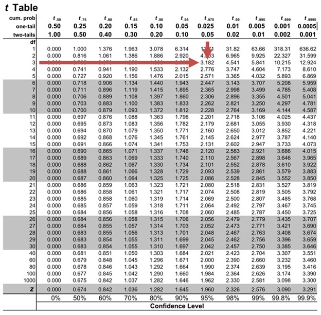
Next, we need to find critical t-values. Note that this is a one-sided test. As such, we need to find \(t_8,0.05\). We will use the t-table:

From the table, \(t_8,0.05=1.860\). We fail to reject the null hypothesis since the calculated test statistic is less than the critical t-value \((−5.193 \lt 1.860)\). There is sufficient evidence to indicate that the slope coefficient is not positive.

Relationship between the Hypothesis Test of Correlation and Slope Coefficient

In simple linear regression, a distinct characteristic exists: the t-test statistic checks if the slope coefficient equals zero. This t-test statistic is the same as the test-statistic used to determine if the pairwise correlation is zero.

This feature is true for two-sided tests \((H_0: \rho = 0 \text{ versus } H_a: \rho \neq 0\) and \(H_0: b_1 = 0 \text{ versus } H_a: \rho \neq 0)\) and one-sided test \((H_0: \rho\le 0 \text{ versus } Ha: \rho> 0\) and \(H_0: b_1\le 0 \text{ versus } H_a: \rho \gt 0\) or \(H_0: \rho \gt 0 \text{ versus } H_a: \rho \le 0\) and \(H_0: b_1 \gt 0 \text{ versus } H_a: \rho \le 0)\).

Note that the test -statistic to test whether the correlation is equal to zero is given by:

$$ t=\frac{r\sqrt{n-2}}{\sqrt{1-r^2}} $$

The above test statistic is t-distributed with \((n-2)\) degrees of freedom.

Consider our previous example, where we regressed inflation rates against unemployment rates from 2011 to 2020. Assume we want to test whether the pairwise correlation between the unemployment and inflation rates equals zero.

In the example, the correlation between the unemployment rates and inflation rates is -0.8782. As such, the test- statistic to test whether the correlation is equal to zero is

$$ t=\frac{-0.8782\sqrt{10-2}}{\sqrt{1-{(-0.8782)}^2}}\approx-5.19 $$

Note this is equal to the test statistic t-test statistic used to perform the hypothesis test whether the slope coefficient is zero:

$$
t=\frac{{\hat{b}}_1-B_1}{s_{{\hat{b}}_1}}=\frac{-0.9020-0}{0.1737}=-5.193 $$

Hypothesis Test of the Intercept Coefficient

Similar to the slope coefficient, we may also want to test whether the population intercept is equal to a certain value. The process is similar to that of the slope coefficient. However, the test statistic for t-distributed test on slope coefficient is given by:

$$ t=\frac{{\hat{b}}_0-B_0}{s_{{\hat{b}}_0}} $$

Where:

\(B_1\) = Hypothesized intercept coefficient.

\(\widehat{b_1}\) = Point estimate for \(b_1\).

\(s_{{\hat{b}}_0}\) = Standard error of the intercept.

The formula for the standard error of the intercept \(s_{{\hat{b}}_0}\) is given by:

$$ s_{{\hat{b}}_0}=\sqrt{\frac{1}{n}+\frac{{\bar{X}}^2}{\sum_{i=1}^{n}\left(X_i-\bar{X}\right)^2}} $$

Recall the example where regressed inflation rates against unemployment rates from 2011 to 2020.

$$ \begin{array}{c|c|c|c|c|c|c|c}
\text{Year} & \text{Unemployment} & \text{Inflation} & \text{Predicted} & \text{Variation} & \text{Variation} & \text{Variation} & (X_i \\
& {\text{Rate } \% (X_i)} & {\text{Rate }\%} & \text{Unemployment} & \text{to be} & \text{Unexplained} & \text{Explained} & -\bar{X})^2 \\
& & ({{Y}}_i) & {\text{rate } (\hat Y_i)} & \text{Explained.} & & & \\
& & & & \left(Y_i-\bar{Y}\right)^2 & \left(Y_i- \hat{Y}_i\right)^2 & \left({\hat{Y}}_i-\bar{Y}\right)^2 & \\ \hline
2011 & 6.1 & 1.7 & 1.610 & 0.410 & 0.008 & 0.533 & 0.656 \\ \hline
2012 & 7.4 & 1.2 & 0.437 & 1.300 & 0.582 & 3.621 & 4.452 \\ \hline
\vdots & \vdots & \vdots & \vdots & \vdots & \vdots & \vdots & \vdots \\ \hline
2019 & 4.0 & 4.7 & 3.504 & 5.570 & 1.430 & 1.355 & 1.664 \\ \hline
2020 & 3.9 & 3.6 & 3.594 & 1.588 & 0.000 & 1.573 & 1.932 \\ \hline
\textbf{Sum} & \bf{52.90} & \bf{23.4} & & \bf{13.704} & \bf{3.136} & \bf{10.568} & \bf{12.989} \\ \hline
\textbf{Arithmetic} & \bf{5.29} & \bf{2.34} & & & & & \\
\textbf{Mean} & & & & & & & \\
\end{array} $$

The estimated regression model is

$$ \hat{Y}=7.112-0.9020X_i+\varepsilon_i $$

Assume that we need to test whether the intercept is greater than 1 at a 5% significance level.

The hypotheses are as follows:

$$ H_0: b_0\le 1 \text{ versus } H_a: b_0 \gt 1 $$

Next, we need to calculate the test statistic given by:

$$ t=\frac{{\hat{b}}_0-B_0}{s_{{\hat{b}}_0}} $$

Where:

$$ s_{{\hat{b}}_0}=\sqrt{\frac{1}{n}+\frac{{\bar{X}}^2}{\sum_{i=1}^{n}\left(X_i-\bar{X}\right)^2}}=\sqrt{\frac{1}{10}+\frac{{5.29}^2}{\sqrt{12.989}}}=2.804 $$

Therefore,

$$ t=\frac{7.112-1}{2.804}=2.180 $$

Note that this is a one-sided test. From the table, \(t_8,0.05=1.860\). Since the calculated test statistic is less than the critical t-value \((2.180 \gt 1.860)\), we reject the null hypothesis. There is sufficient evidence to indicate that the intercept is greater than 1.

Hypothesis Tests Concerning Slope Coefficient When Independent Variable is an Indicator Variable

Dummy variables, also known as indicator variables or binary variables, are used in regression analysis to represent categorical data with two or more categories. They are particularly useful for including qualitative information in a model that requires numerical input variables.

Example: Regression Analysis With Indicator Variables

Assume we aim to investigate if a stock’s inclusion in an Environmental, Social, and Governance (ESG) focused fund affects its monthly stock returns. In this case, we’ll analyze the monthly returns of a stock over a 48-month period.

We can use a simple linear regression model to explore this. In the model, we regress monthly returns, denoted as R, on an indicator variable, ESG. This indicator takes the value of 0 if the stock isn’t part of an ESG-focused fund and 1 if it is.

$$ R=b_0+b_1ESG+\varepsilon_i $$

Note that we estimate the simple linear regression in a way similar to if the independent variable was continuous.

The intercept \(\beta_0\) is the predicted value when the indicator variable is 0. On the other hand, the slope when the indicator variable is 1 is the difference in the means if we grouped the observations by the indicator variable.

Assume that the following table is the results of the above regression analysis:

$$ \begin{array}{c|c|c|c}
& \textbf{Estimated} & \textbf{Standard Error} & \textbf{Calculated Test} \\
& \textbf{Coefficients} & \textbf{of Coefficients} & \textbf{Statistic} \\ \hline
\text{Intercept} & 0.5468 & 0.0456 & 9.5623 \\ \hline
\text{ESG} & 1.1052 & 0.1356 & 9.9532
\end{array} $$

Additionally, we have the following information regarding the means and variances of the variables.

$$ \begin{array}{c|c|c|c}
& \textbf{Monthly returns} & \textbf{Monthly Returns} & \textbf{Difference in} \\
& \textbf{of ESG Focused} & \textbf{of Non-ESG} & \textbf{Means} \\
& \textbf{Stocks} & \textbf{Stocks} & \\ \hline
\text{Mean} & 1.6520 & 0.5468 & 1.1052 \\ \hline
\text{Variance} & 1.1052 & 0.1356 & \\ \hline
\text{Observations} & 10 & 38 &
\end{array} $$

From the above tables, we can see that:

• The intercept (0.5468) is equal to the mean of the returns for the non-ESG stocks.
• The slope coefficient (1.1052) is the difference in means of returns between ESG-focused stocks and non-ESG stocks.

Now, assume that we want to test whether the slope coefficient is equal to 0 at a 5% significance level. Therefore, the hypothesis is \(H_0:\beta_1=0 \text{ vs. } H_a:\beta_1\neq0\). Note that the degrees of freedom in \(48-2=46\). As such, the critical t-values (usually given in the table above) is \(t_{46,0.025}=\pm2.013\).

From the first table above, the calculated test statistic for the slope is greater than the critical t-value \((9.9532 \gt 2.013)\). As a result, we reject the null hypothesis that the slope coefficient is equal to zero.

p-Values and Level of Significance

The p-value is the smallest level of significance level at which the null hypothesis is rejected. Therefore, the smaller the p-value, the smaller the probability of rejecting the true null hypothesis (type I error) and, hence, the greater the validity of the regression model.

Software packages commonly offer p-values for regression coefficients. These p-values help test a null hypothesis that the true parameter equals 0 versus the alternative that it’s not equal to zero.

We reject the null hypothesis if the p-value corresponding to the calculated test statistic is less than the significance level.

Example: Hypothesis Testing of Slope Coefficients

An analyst generates the following output from the regression analysis of inflation on unemployment:

$$\small{\begin{array}{llll}\hline{}& \textbf{Regression Statistics} &{}&{}\\ \hline{}& \text{R Square} & 0.7684 &{} \\ {}& \text{Standard Error} & 0.0063 &{}\\ {}& \text{Observations} & 10 &{}\\ \hline {}& & & \\ \hline{} & \textbf{Coefficients} & \textbf{Standard Error} & \textbf{t-Stat}\\ \hline \text{Intercept} & 0.0710 & 0.0094 & 7.5160 \\\text{Forecast (Slope)} & -0.9041 & 0.1755 & -5.1516\\ \hline\end{array}}$$

At the 5% significant level, test the null hypothesis that the slope coefficient is significantly different from one, that is,

$$ H_{0}: b_{1} = 1 \text{ vs. } H_{a}: b_{1} \neq 1 $$

Solution

The calculated t-statistic, \(\text{t}=\frac{\hat{b}_{1}-b_1}{\hat{S}_{b_{1}}}\) is equal to:

$$\begin{align*} {t}= \frac{-0.9041-1}{0.1755} = -10.85\end{align*}$$

The critical two-tail t-values from the table with \(n-2=8\) degrees of freedom are:

$$ {t}_{c}=\pm 2.306$$

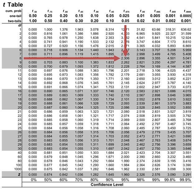
Notice that \(|t| \gt t_{c}\) i.e., (\(10.85 \gt 2.306\))

Therefore, we reject the null hypothesis and conclude that the estimated slope coefficient is statistically different from one.
Note that we used the confidence interval approach and arrived at the same conclusion.

Question 1

Samantha Lee, an investment analyst, is studying monthly stock returns. She focuses on companies listed in a Renewable Energy Index across various economic conditions. In her analysis, she performed a simple regression. This regression explains how stock returns vary concerning the indicator variable RENEW. RENEW equals 1 when there’s a positive policy change towards renewable energy during that month, and 0 if not. The total variation in the dependent variable amounted to 220.34. Of this, 94.75 is the part explained by the model. Samantha’s dataset includes 36 monthly observations.

Calculate the coefficient of determination, F-statistic, and standard deviation of monthly stock returns of companies listed in a Renewable Energy Index.

1. \(R^2\)=43.00%;F=26.07;Standard deviation=2.51.
2. \(R^2\)=53.00%;F=26.41;Standard deviation=2.55.
3. \(R^2\)=33.00%;F=36.07;Standard deviation=3.55.

Solution

The correct answer is A.

Coefficient of determination:

$$ R^2=\frac{\text{Explained variation}}{\text{Total variation}}=\frac{94.75}{220.34}\approx43\% $$

F-statistic:

$$ F=\frac{\frac{\text{Explained variation}}{k} }{\frac{\text{Unexplained variation}}{n-2}}=\frac{\frac{SSR}{k}}{\frac{SSE}{n-2}} =\frac{\frac{94.75}{1}}{\frac{220.34-94.75}{34}}=26.07 $$

Standard deviation:

Note that,

$$ \text{Total Variation}= \sum_{i=1}^{n}{\left(Y_i-\bar{Y}\right)^2=220.34} $$

And the standard deviation is given by:

$$ \text{Standard deviation}=\sqrt{\frac{\sum_{i=1}^{n}\left(Y_i-\bar{Y}\right)^2}{n-1}} $$

As such,

$$ \text{Standard deviation}=\sqrt{\frac{\text{Total variation}}{n-1}}=\sqrt{\frac{220.34}{n-1}}=2.509 $$

Question 2

Neeth Shinu, CFA, is forecasting the price elasticity of supply for a specific product. Shinu uses the quantity of the product supplied for the past 5months as the dependent variable and the price per unit of the product as the independent variable. The regression results are shown below.

$$\small{\begin{array}{lccccc}\hline \textbf{Regression Statistics} & & & & & \\ \hline \text{R Square} & 0.9941 & & & \\ \text{Standard Error} & 3.6515 & & & \\ \text{Observations} & 5 & & & \\ \hline {}& \textbf{Coefficients} & \textbf{Standard Error} & \textbf{t Stat} & \textbf{P-value}\\ \hline\text{Intercept} & -159 & 10.520 & (15.114) & 0.001\\ \text{Slope} & 0.26 & 0.012 & 22.517 & 0.000\\ \hline\end{array}}$$

Which of the following most likely reports the correct value of the t-statistic for the slope and most accurately evaluates its statistical significance with 95% confidence?

1. \(t=21.67\); the slope is significantly different from zero.
2. \(t= 3.18\); the slope is significantly different from zero.
3. \(t=22.57\); the slope is not significantly different from zero.

Solution

The correct answer is A.

The t-statistic is calculated using the formula:

$$\text{t}=\frac{\hat{b}_{1}-b_1}{\hat{S}_{b_{1}}}$$

Where:

• \(b_{1}\) = True slope coefficient.
• \(\hat{b}_{1}\) = Point estimator for \(B_{1}\).
• \(\hat{S}_{b_{1}}\) = Standard error of the regression coefficient.

$$\begin{align*} {t}=\frac{0.26-0}{0.012}=21.67\end{align*}$$

The critical two-tail t-values from the t-table with \(n-2 = 3\) degrees of freedom are:

$$t_{c}= \pm 3.18 $$

Notice that \(|t| \gt t_{c}\) (i.e., \(21.67 \gt 3.18\)).

Therefore, the null hypothesis can be rejected. Further, we can conclude that the estimated slope coefficient is statistically different from zero.