Measures of Central Tendency and Location

The center of any data is identified via a measure of central tendency. A measure of central tendency for a series of returns reveals the center of the empirical distribution of returns. They include mean, mode, and median.

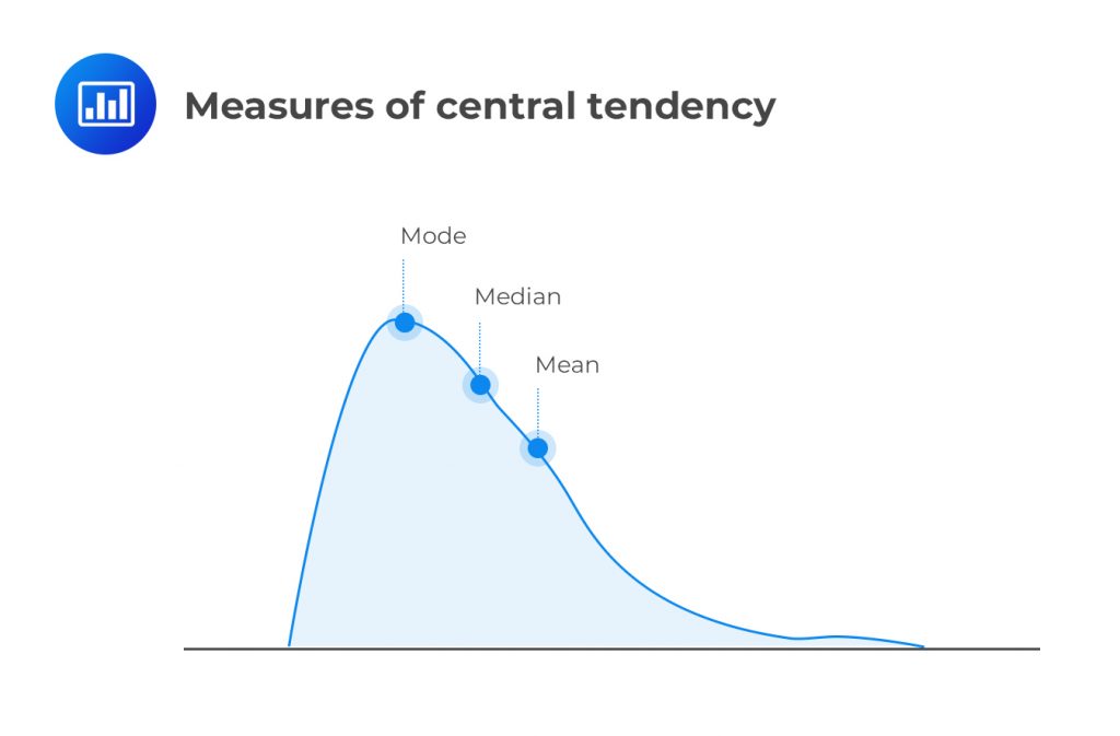
Measures of location help us understand where data points tend to cluster. These measures include central tendency measures such as mean, median, and mode. There are also other measures that provide different insights into how the data is spread out or located within a distribution.

Measures of Central Tendency

Arithmetic Mean

The arithmetic mean is the sum of the values of the observations in a dataset divided by the number of observations.

Recall the formula: denoted by \( {\bar{R}}_i\) arithmetic mean for an asset i is a simple process of finding the average holding period returns. It is given by:

$${\bar{R}}_i=\frac{R_{i,1}+R_{i,1}+\ldots+R_{i,T-1}+R_{iT}}{T}=\frac{1}{T}\sum_{t=1}^{T}R_{it}$$

Where:

\(R_{it}\) = Return of asset i in period t.

\(T\) = Total number of periods.

For example, if a share has returned 15%, 10%, 12%, and 3% over the last four years, then the arithmetic mean is computed as follows:

$${\bar{R}}_i=\frac{1}{T}\sum_{t=1}^{T}R_{it}=\frac{1}{4}\left(15\%+10\%+12\%+3\%\right)=10\%$$

Population Mean and Sample Mean

The population mean is the summation of all the observed values in the population, \(\sum X_i\) divided by the total number of observations, \(N\). The population mean differs from the sample mean, which is based on a few observed values chosen from the population. Thus:

$$\begin{align}\text{Population mean}&=\ \frac{\sum X_i}{N}\\ \text{ Sample mean}&=\ \frac{\sum X_i}{n}\end{align}$$

Analysts use the sample mean to estimate the actual population mean.

The population mean and the sample mean are both arithmetic means. The arithmetic mean for any data set is unique and is computed using all the data values. Among all the measures of central tendency, it is the only measure for which the sum of the deviations from the mean is zero.

Example: Calculating the Arithmetic Mean

The following are the annual returns realized from a given asset between 2005 and 2015.

{12%   13%   11.5%   14%   9.8%   17%   16.1%   13%   11%   14%}

Calculate the population mean.

Solution

$$\begin{align}\text{Population mean}&=\frac{0.12+0.13+0.115+0.14+0.098+0.17+0.161+0.13+0.11+0.14}{10} \\&=\ 0.1314 =\ 13.14\% \end{align}$$

Median

The median is the statistical value located at the center of a data set organized in ascending or descending order.

Consider a sample of n observations. For an odd-numbered of observations, the median is the observation that is located in \(\frac{(n+1)}{2}\) position. On the other hand, if the number of observations is even, the media is the mean value of the observations located in \(\frac{n}{2}\) and \(\frac{n+2}{2}\) position.

Unlike the arithmetic mean, the median resists the effects of extreme observations. However, it only gives the relative position of the ranked observations without considering all observations relating to the size of the observations.

Example: Calculating the Median

The following are the annual returns on a given asset realized between 2005 and 2015.

{12%   13%   11.5%   14%   9.8%   17%   16.1%   13%   11%   14%}

The median is closest to:

Solution

First, we arrange the returns in ascending order:

{9.8%   11%   11.5%   12%   13%   13%   14%   14%   16.1%   17%}

Since the number of observations is even, the median return will be the middle point of the two middle values in the positions \(\frac{n}{2}\) and \(\frac{(n+2)}{2}\).

The value occupying \(\frac{n}{2}=\frac{10}{5}\) = 5th position is 13, and the value located in \(\frac{(n+2)}{2}=\frac{12}{2}\) = 6th position is 13, so that the mode is:

$$\frac{13\%+13\%}{2}=13\%$$

Mode

The mode is the value that appears most often in a dataset. Sometimes, a dataset has a mode; sometimes, it doesn’t. If all the observations in a dataset are different and no value repeats more than others, then the dataset has no mode.

A dataset with one mode is called unimodal. When there are two modes, it’s called bimodal. If the distribution has three frequently occurring values, it’s termed trimodal.

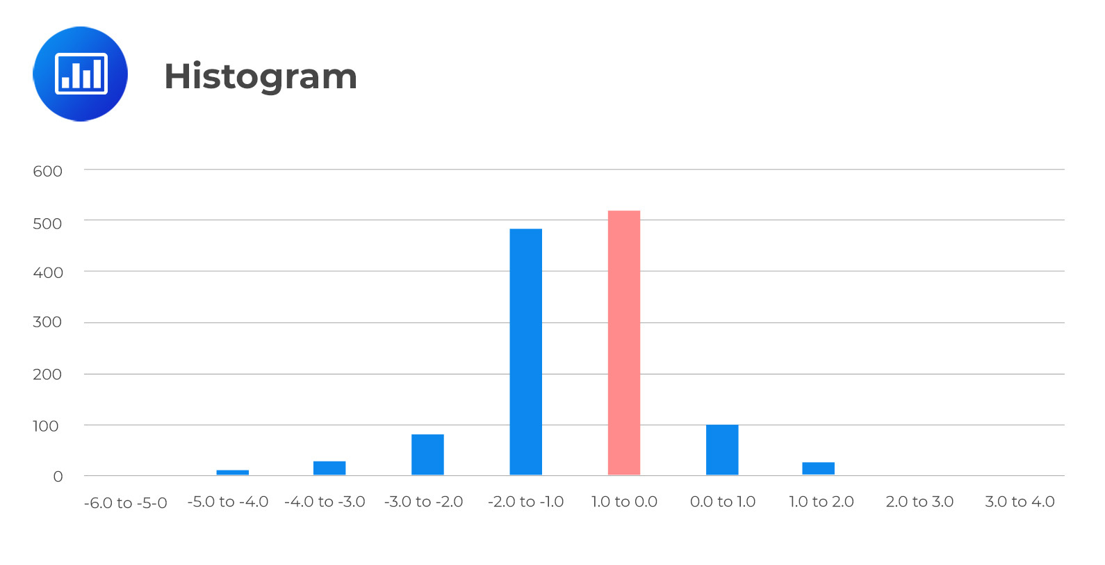
An interval with the highest frequency is called the modal interval (or intervals) in a frequency distribution. For instance, in the frequency distribution below, the modal interval is \(\textbf{-1.0 to 0.0}\) with an absolute frequency of 520.

$$\begin{array}{c|c|c|c|c}  \textbf{Return Bin} & \textbf{Absolute} & \textbf{Relative}  & \textbf{Cumulative} & \textbf{Cumulative}]\\  \textbf{(%)}&\textbf{ Frequency}&\textbf{Frequency(%)}&\textbf{Absolute}&\textbf{Relative}\\  {}&{}&{}&\textbf{Frequency}&\textbf{Frequency (%)}\\ \hline \text{-6.0 to -5.0} & 2 & 0.16 & 2 & 0.16 \\ \text{-5.0 to -4.0} & 8 & 0.64 & 10 & 0.80 \\ \text{-4.0 to -3.0} & 27 & 2.16 & 37 & 2.96 \\ \text{-3.0 to -2.0} & 80 & 6.40 & 117 & 9.36 \\ \text{-2.0 to -1.0} & 485 & 38.80 & 602 & 48.16 \\ \textbf{-1.0 to 0.0} & \textbf{520} & 41.60 & 1,122 & 89.76 \\ \text{0.0 to 1.0} & 100 & 8.00 & 1,222 & 97.76 \\ \text{1.0 to 2.0} & 24 & 1.92 & 1,246 & 99.68 \\ \text{2.0 to 3.0} & 3 & 0.24 & 1,249 & 99.92 \\ \text{3.0 to 4.0} & 1 & 0.08 & 1,250 & 100.00 \\ \hline \end{array}$$

In a histogram, the modal interval always has the highest bar.

The mode is the only measure of central tendency that can be used with nominal data. Nominal data refers to a type of data that is categorized into distinct categories or groups without any inherent order or numerical value. Examples of nominal data include gender (male, female), eye color (blue, brown, green), and marital status (single, married, divorced).

Example: Calculating the Mode

Determine the mode from the following data set:

{20%   23%   20%   16%   21%   20%   16%   23%   25%   27%   20%}

Solution

The mode is 20%. It occurs four times, a frequency higher than any other value in the data set. Clearly, this dataset is unimodal.

Dealing With Outliers

An outlier may represent a distinct value in a population. In addition, it may show that there was an error in recording the value, or it was generated from a different population.

When working with a sample with outliers, we can potentially transform the variable or choose another variable that achieves the same objective. If these observations prove to be impossible, there are three options:

Option 1: Take no action and use the data as it is. If these observations are accurate, then this is appropriate.

Option 2: Remove outliers using the trimmed mean. For example, when calculating the central tendency, a 4 percent trimmed mean excludes the lowest 2% and highest 2% of values.

Option 3: Substitute a different value for the outliers. The winsorized mean is an illustration of a central tendency that does this. For instance, when computing a 96% winsorized mean, the value at or above the lowest and highest 2% is assigned the lowest and highest 2% values.

Measures of Location

Quartiles, quintiles, deciles, and percentiles are values or cut points that partition a finite number of observations into nearly equal-sized subsets. The number of partitions depends on the type of cut point involved.

Quartiles

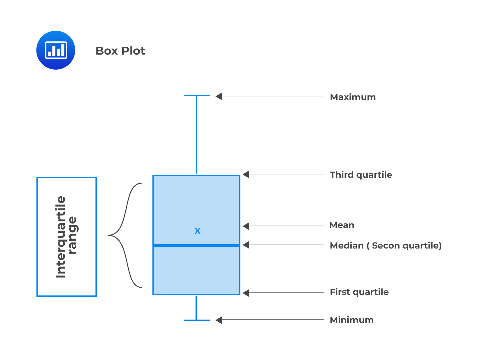
They divide data into four parts. The first quartile, Q₁, is referred to as the lower quartile, and the last quartile, Q_4, is the upper quartile. Q₁ splits the data into the lower 25% and upper 75% values. Similarly, the upper quartile subdivides the data into the lower 75% of the values and the upper 25%. The difference between the upper and lower quartiles is known as the interquartile range, which indicates the spread of the middle 50% of the data.

Quintiles

Though rarely used in practice, quintiles split a set of data into five equal parts, i.e., fifths. Therefore, the second quintile splits data into the lower 40% of the values and the upper 60%.

Deciles

The deciles subdivide data into ten equal parts. There are 10 deciles in any data set. For example, the fourth decile splits data into the lower 40% of the values and the upper 60%.

Percentiles

Percentiles split data into 100 equal parts, i.e., hundredths. So, for instance, the 77^th percentile splits the data into the lower 77% of the values and the upper 23%.

Financial analysts commonly use the four types of subdivisions to rank investment performance. You should note that quartiles, quintiles, and deciles can all be expressed as percentiles. For instance, the first quartile is just the 25^th percentile. Similarly, the fourth decile is simply the 40^th percentile. This enables the application of the formula below.

$$\text{Position of percentile}=\frac{\left(n+1\right)y}{100}$$

Example:  Calculating Quartiles

Given the following distribution of returns, calculate the lower quartile.

{10%   23%   12%   21%   14%   17%   16%   11%   15%   19%}

Solution

First, we have to arrange the values in ascending order:

{10%   11%   12%   14%   15%   16%   17%   19%    21%   23%}

Next, we establish the position of the first quartile. This is simply the 25^th percentile. Therefore:

$$P_{25}=\frac{\left(10+1\right)25}{100}={2.75}^{th}\ value$$

Since the value is not straightforward, we have to extrapolate between the 2^nd and the 3^rd data points. The 25^th percentile is three-fourths (0.75) of the way from the 2^nd data point (11%) to the 3^rd data point (12%):

$$11\%+0.75\times\left(12-11\right)=11.75\%$$

Box and Whisker Plot

Box and whisker plot is used to display the dispersion of data across quartiles. A box and whisker plot consists of a “box” with “whiskers” connected to the box. It shows the following five-number summary of a set of data.

Example: Box and Whisker Plot

Consider the following box and whisker plot:

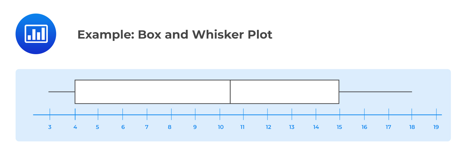
1. Which of the following is most likely the median?

A. 10.

B. 5.

C. 11.

Solution

The correct answer is B.

$$\text{Median or Quartile 2 (Q2) = \frac{\left(10+11\right)}{2}=10.5$$

2. Which of the following is most likely the interquartile range?

A. 4.5.

B. 6.5.

C. 11.

Solution

The correct answer is C.

$$\text{Interquartile range is}\ Q_3-Q_1=15-4=11$$

3. Which of the following is most likely the 3^rd quartile?

A. 4.

B. 15.

C. 18.

Solution

$$\text{Quartile 3 (Q3)} = \frac{3\times\left(n+1\right)}{4}=\ \frac{3\times\left(16+1\right)}{4}=12.75th\ \text{term, which is}\ 14.75$$

Quantiles in Investment Practice

Quantiles have two main purposes in investment practice. First, quantiles are used to rank performance. Secondly, quantiles can be used in investment research for comparison purposes. For example, companies can be clustered into deciles to compare the performance of small companies with the large ones. In this case, the first decile will contain the portfolio of companies with the smallest market values, while the tenth decile will contain the companies with the largest market values.

Question

A mutual fund achieved the following rates of growth over an 11-month period:

{3%   2%   7%   8%   2%   4%   3%   7.5%   7.2%   2.7%   2.09%}

The 5^th decile from the data is closest to:

A. 2%.

B. 3%.

C. 4%.

Solution

The correct answer is B.

First, you should re-arrange the data in ascending order:

{2%   2% 2.09% 2.7%    3%   3%   4%   7%   7.2%   7.5%   8%}

Secondly, you should establish the 5^th decile. This is simply the 50^th percentile and is actually the median:

$$\begin{align}P_{50}&=\frac{\left(1+11\right)50}{100}\\& =12\times 0.5\\& =6,\ \text{i.e., the 6th data point}\end{align}$$

Therefore, the 5th decile = 50th percentile = Median = 3%