Assume that we have samples of size \(n\) for dependent variable \(Y\) and independent variable \(X\). We wish to estimate the simple regression of \(Y\) and \(X\). The classic normal linear regression model assumptions are as follows:
-
-
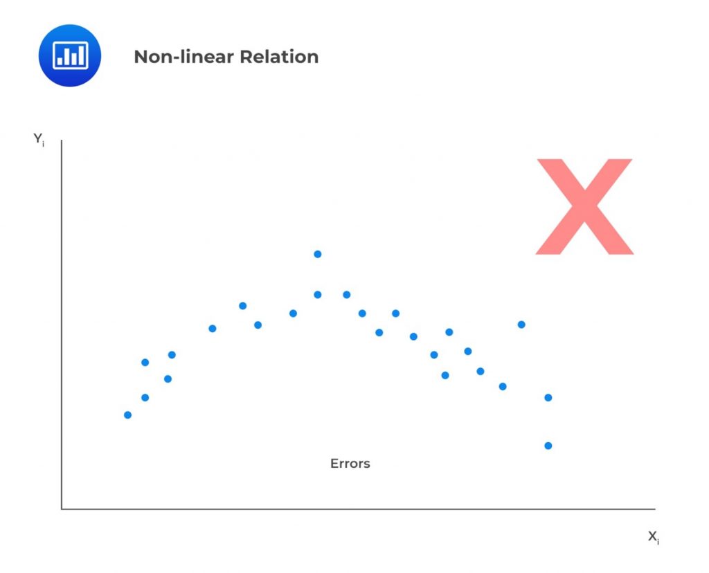
- Linearity: A linear relationship implies that the change in \(Y\) due to a one-unit change in \(X\) is constant, regardless of the value \(X\) takes. If the relationship between the two is not linear, the regression model will not accurately capture the trend, resulting in inaccurate predictions. The model will be biased and underestimate or overestimate \(Y\) at various points. For example, the model \(Y=b_0+b_1e^{b_1x}\) is nonlinear in \(b_1\). For this reason, we should not attempt to fit a linear model between \(X\) and \(Y\). It also follows that the independent variable, \(X\), must be non-stochastic (must not be random). A random independent variable rules out a linear relationship between the dependent and independent variables. In addition, linearity means the residuals should not exhibit an observable pattern when plotted against the independent variable. Instead, they should be completely random. In the example below, we’re looking at a scenario where the residuals appear to show a pattern when plotted against the independent variable, \(X\). This effectively indicates a nonlinear relation.

- Normality Assumption: This assumption implies that the error terms (residuals) must follow a normal distribution. It’s important to note that this doesn’t mean the dependent and independent variables must be normally distributed. However, checking the distribution of the dependent and independent variables is crucial to identify any outliers. A histogram of the residuals can be used to detect if the error term is normally distributed. A symmetric bell-shaped histogram indicates that the normality assumption is likely to be true.
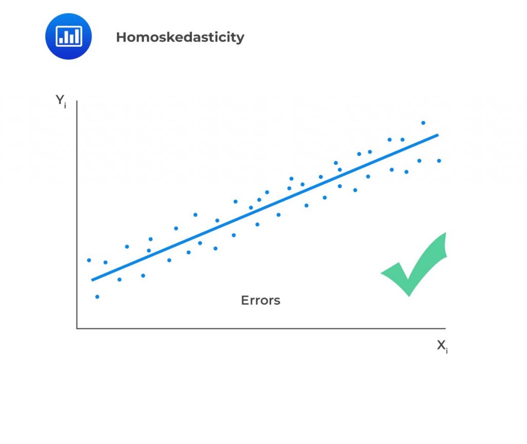
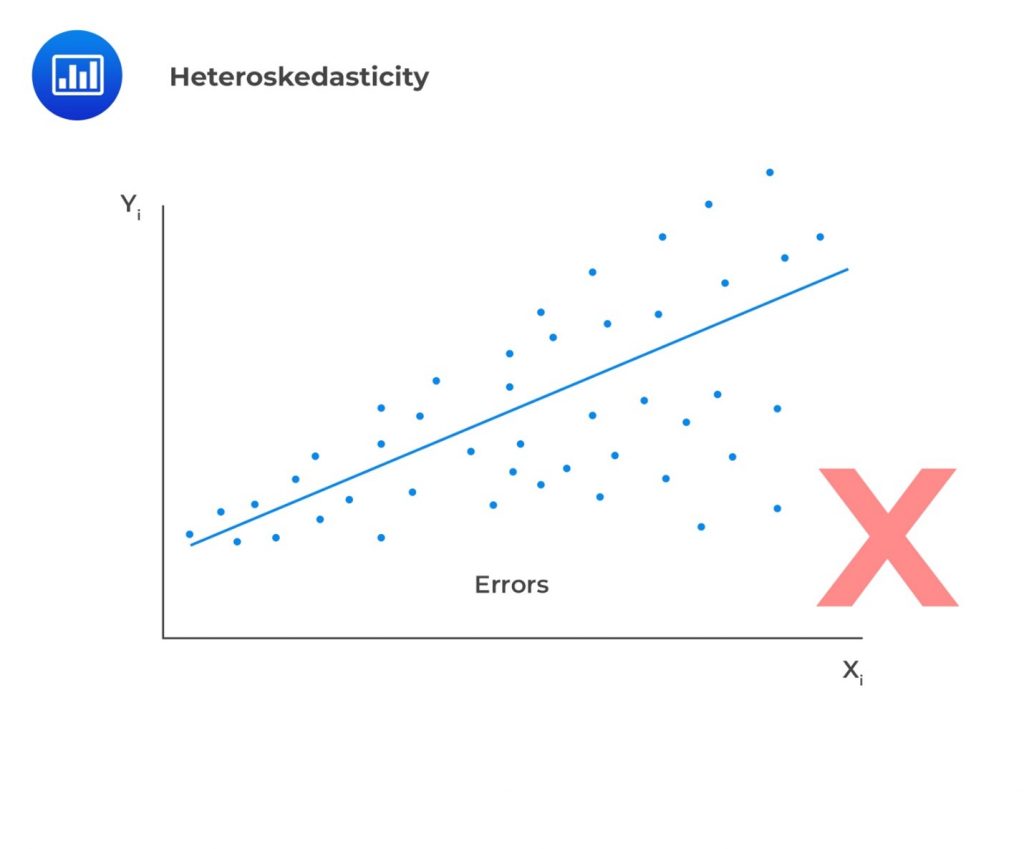
- Homoskedasticity: Homoskedasticity implies that the variance of the error terms is constant across all observations. Mathematically, this is expressed as:$$ E\left(\epsilon_i^2\right)=\sigma_\epsilon^2,\ \ i=1,2,\ldots,n $$If the variance of residuals varies across observations, then we refer to this as heteroskedasticity (not homoscedasticity). We plot the least square residuals against the independent variable to test for heteroscedasticity. If there is an evident pattern in the plot, that is a manifestation of heteroskedasticity.

In case residuals and the predicted values increase simultaneously, then such a situation is known as heteroscedasticity (or heteroskedasticity).

- Independence Assumption: The independence assumption implies that the observations \(X_i\) and \(Y_i\) are independent of each other. Failure to satisfy this assumption implies the variables are not independent, and thus, residuals will be correlated. To ascertain this assumption, we visually and statistically analyze the residuals to check whether residual shows exhibit a pattern.
Question
A regression model with one independent variable requires several assumptions for valid conclusions. Which of the following statements most likely violates those assumptions?
- The independent variable is random.
- The error term is distributed normally.
- There exists a linear relationship between the dependent variable and the independent variable.
Solution
The correct answer is A.
Linear regression assumes that the independent variable, X, is NOT random. This ensures that the model produces the correct estimates of the regression coefficients.
B is incorrect. The assumption that the error term is distributed normally allows us to easily test a particular hypothesis about a linear regression model.
C is incorrect. Essentially, the assumption that the dependent and independent variables have a linear relationship is the key to a valid linear regression. If the parameters of the dependent and independent variables are not linear, then the estimation of that relation can yield invalid results.
