Introduction to Linear Regression

Linear regression is a mathematical method used for analyzing how the variation in one variable can explain the variation in another variable.

Let \(Y\) be the variable we wish to explain. As such, the observation of this variable is \(Y_i\), and \(\bar{Y}\) is the mean of the sample size \(n\). The variation of \(Y\) is given by:

$$ \text{Variation of } Y= \sum_{i=1}^{n}\left(Y_i-\bar{Y}\right)^2 $$

Our main objective is to explain what causes this variation, usually called the sum of squares total (SST).

By definition of the regression, we need to explain the variation of \(Y\) with another variable. Let \(X\) be the explanatory variable. As such, the observations of \(X\) will be denoted by \(X_i\) and \(\bar{X}\) sample mean of size \(n\). The variation of X is given by:

$$ \text{Variation of } X= \sum_{i=1}^{n}\left(X_i-\bar{X}\right)^2 $$

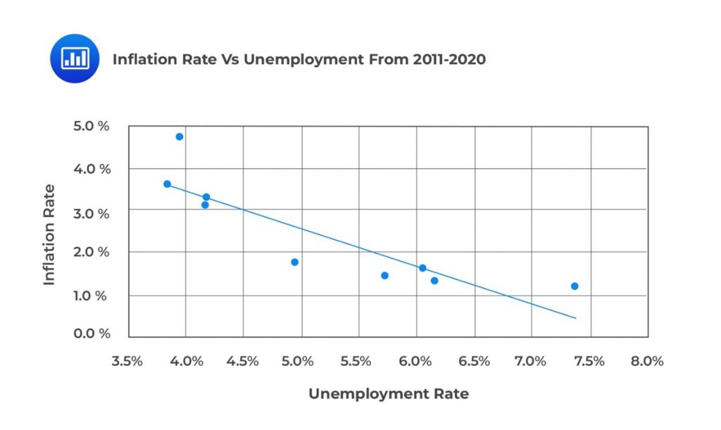
To visualize the relationship between variables X and Y, you can use a scatter plot, also known as a scattergram. In this type of plot, the variable you want to explain (Y) is usually plotted on the vertical axis. In contrast, the explanatory variable (X) is placed on the horizontal axis to show the relationship between their variations.

For example, consider the following table. We wish to use linear regression analysis to forecast inflation, given unemployment data from 2011 to 2020.

$$ \begin{array}{c|c|c}
\text{Year} & \text{Unemployment Rate} & \text{Inflation Rate} \\ \hline
2011 & 6.1\% & 1.7\% \\ \hline
2012 & 7.4\% & 1.2\% \\ \hline
2013 & 6.2\% & 1.3\% \\ \hline
2014 & 6.2\% & 1.3\% \\ \hline
2015 & 5.7\% & 1.4\% \\ \hline
2016 & 5.0\% & 1.8\% \\ \hline
2017 & 4.2\% & 3.3\% \\ \hline
2018 & 4.2\% & 3.1\% \\ \hline
2019 & 4.0\% & 4.7\% \\ \hline
2020 & 3.9\% & 3.6\%
\end{array} $$

In this scenario, the \(Y\) variable is the inflation rate, and the \(X\) axis is the unemployment rate. A scatter plot of the inflation rates against unemployment rates from 2011 to 2020 is shown in the following figure.

Dependent and Independent Variables

A dependent variable, often denoted as $Y$, is the variable we want to explain. In contrast, an independent variable, typically denoted as $X$, is used to explain variations in the dependent variable. The independent variable is also referred to as the exogenous, explanatory, or predicting variable.

In our example above, the dependent variable is the inflation rate, and the independent variable is the unemployment rate.

To understand the relationship between dependent and independent variables, we estimate a linear relationship, usually a straight line. When there’s one independent variable, we use simple linear regression. If there are multiple independent variables, we use multiple regression.

This reading focuses on linear regression.

Least Squares Criterion

In simple linear regression, we assume linear relationships exist between the dependent and independent variables. The aim is to fit a line to the observations of X \((X_is)\) and Y \((Y_is)\) to minimize the squared deviations from the line. To accomplish this, we use the least squares criterion.

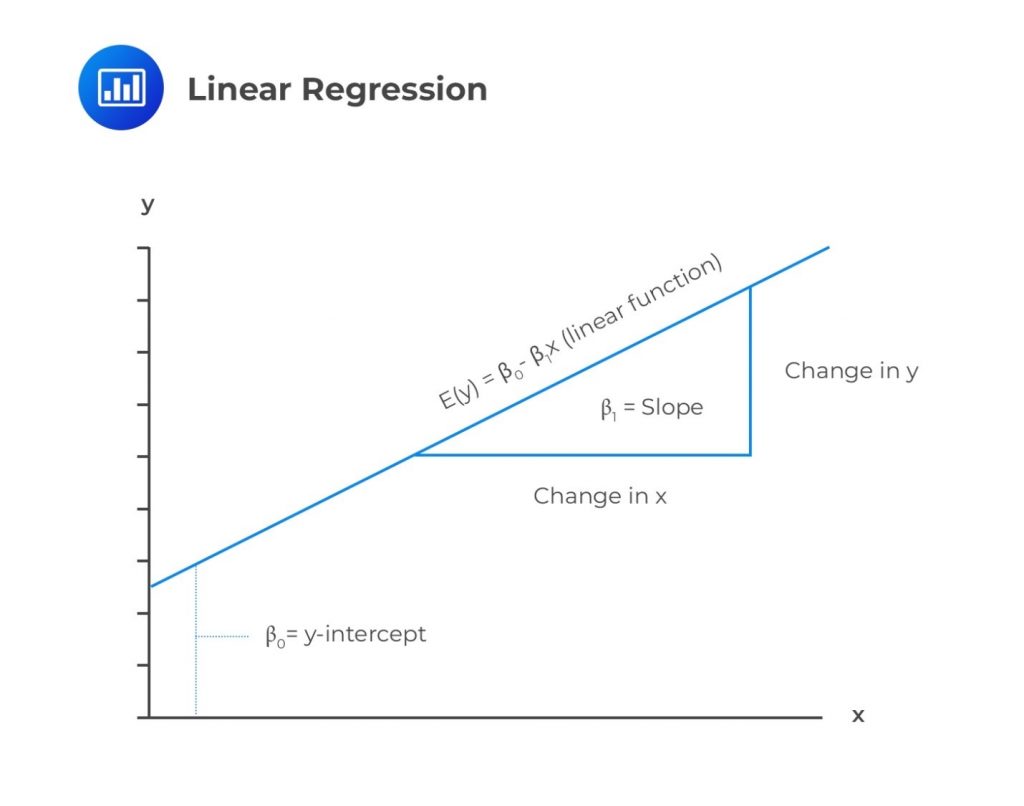
The following is a simple linear regression equation:

$$ Y=b_0+b_1X_1+\varepsilon_i,\ \ i=1,2,\ldots,n $$

Where:

\(Y\) = Dependent variable.

\(b_0\) = Intercept.

\(b_1\) = Slope coefficient.

\(X\) = Independent variable.

\(\varepsilon\) = Error term (Noise).

\(b_0\) and \(b_1\) are known as regression coefficients. The equation above implies that the dependent is equivalent to the intercept \((b_0)\) plus the product of the slope coefficient \((b_1)\) and the independent variable plus the error term.

The error term is equal to the difference between the observed value of \(Y\) and the one expected from the underlying population relation between \(X\) and \(Y\)

Below is an illustration of a simple linear regression model.

As stated earlier, linear regression calculates a line that best fits the observations. In the following image, the line that best fits the regression is clearly the blue one: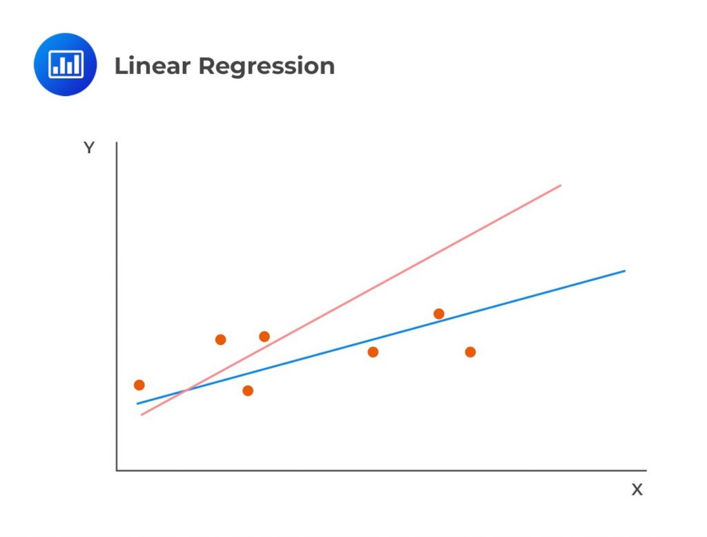

Note that we cannot directly observe the population parameters \(b_0\) and \(b_1\). As such, we observe their estimates, \({\hat{b}}_0\) and \({\hat{b}}_1\). They are the estimated parameters of the population using a sample. In simple linear regression, \({\hat{b}}_0\) and \({\hat{b}}_1\) are such that the sum of squared vertical distances is minimized.

Specifically, we concentrate on the sum of the squared differences between observations \(Y_i\) and the respective estimated value \({\hat{Y}}_i\) on the regression line, also called the sum of squares error (SSE).

Note that,

$$ {\hat{Y}}_i={\hat{b}}_0+{\hat{b}}_1X_i+e_i^2 $$

As such,

$$ SSE=\sum_{i=1}^{n}\left(Y_i-{\hat{b}}_0-{\hat{b}}_1X_i\right)^2=\sum_{i=1}^n{(Y_i-\hat Y_i)}^2=\sum_{i=1}^n e_i^2 $$

Note that the residual for the ith observation \((e_i=Y_i-\hat{Y}_i)\) is different from the error term \((\varepsilon_i)\). The error term is based on the underlying population, while the residual term results from regression analysis on a sample.

Conventionally, the sum of the residuals is zero. As such, the aim is to fit the regression line in a simple linear regression that minimizes the sum of squared residual terms.

Estimation and Interpretation of Regression Coefficients

The Slope Coefficient \({\hat{{\beta}}}_{1}\)

For a simple linear regression, the slope coefficient is estimated as the ratio of the \(Cov(X, Y)\) and \(Var (X)\):

$$
{\hat{b}}_1=\frac{Cov\left(X,Y\right)}{Var\left(X\right)}=\frac{\frac{\sum_{i=1}^{n}\left(Y_i-\bar{Y}\right)\left(X_i-\bar{X}\right)}{n-1}}{\frac{\sum_{i=1}^{n}\left(X_i-\bar{X}\right)^2}{n-1}}=\frac{\sum_{i=1}^{n}\left(Y_i-\bar{Y}\right)\left(X_i-\bar{X}\right)}{\sum_{i=1}^{n}\left(X_i-\bar{X}\right)^2} $$

The slope coefficient is defined as the change in the dependent variable caused by a one-unit change in the value of the independent variable.

The Intercept \({\hat{{\beta}}}_{0}\)

The intercept is estimated using the mean of \(X\) and \(Y\) as follows:

$$ {\hat{b}}_0=\bar{Y}-{\hat{b}}_1\bar{X} $$

Where:

\(\hat{Y}\) = Mean of \(Y\).

\(\hat{X}\) = Mean of \(X\).

The intercept is the estimated value of the dependent variable when the independent variable is zero. The fitted regression line passes through the point equivalent to the means of the dependent and the independent variables in a linear regression model.

Example: Estimating Regression Line

Let us consider the following table. We wish to estimate a regression line to forecast inflation given unemployment data from 2011 to 2020.

$$ \begin{array}{c|c|c}
\text{Year} & {\text{Unemployment Rate}\% \ (X_is)} & {\text{Inflation Rate}\% \ (Y_is)} \\ \hline
2011 & 6.1 & 1.7 \\ \hline
2012 & 7.4 & 1.2 \\ \hline
2013 & 6.2 & 1.3 \\ \hline
2014 & 6.2 & 1.3 \\ \hline
2015 & 5.7 & 1.4 \\ \hline
2016 & 5.0 & 1.8 \\ \hline
2017 & 4.2 & 3.3 \\ \hline
2018 & 4.2 & 3.1 \\ \hline
2019 & 4.0 & 4.7 \\ \hline
2020 & 3.9 & 3.6
\end{array} $$

We can create the following table:

$$ \begin{array}{c|c|c|c|c|c}
\text{Year} & \text{Unemployment} & \text{Inflation} & \left(Y_i-\bar{Y}\right)^2 & \left(X_i-\bar{X}\right)^2 & (Y_i-\bar{Y}) \\
& {\text{Rate}\% \ (X_is)} & { \text{Rate}\% \ (Y_is)} & & & (X_i-\bar{X}) \\ \hline
2011 & 6.1 & 1.7 & 0.410 & 0.656 & -0.518 \\ \hline
2012 & 7.4 & 1.2 & 1.300 & 4.452 & -2.405 \\ \hline
2013 & 6.2 & 1.3 & 1.082 & 0.828 & -0.946 \\ \hline
2014 & 6.2 & 1.3 & 1.082 & 0.828 & -0.946 \\ \hline
2015 & 5.7 & 1.4 & 0.884 & 0.168 & -0.385 \\ \hline
2016 & 5.0 & 1.8 & 0.292 & 0.084 & 0.157 \\ \hline
2017 & 4.2 & 3.3 & 0.922 & 1.188 & -1.046 \\ \hline
2018 & 4.2 & 3.1 & 0.578 & 1.188 & -0.828 \\ \hline
2019 & 4.0 & 4.7 & 5.570 & 1.664 & -3.044 \\ \hline
2020 & 3.9 & 3.6 & 1.588 & 1.932 & -1.751 \\ \hline
\textbf{Sum} & \bf{52.90} & \bf{ 23.4} & \bf{13.704} & \bf{12.989} & \bf{-11.716} \\ \hline
\textbf{Arithmetic} & \bf{5.29} & \bf{2.34} & & & \\
\textbf{Mean}
\end{array} $$

From the table above, we estimate the regression coefficients:

$$ \begin{align*} {\hat{b}}_1 & =\frac{Cov\left(X,Y\right)}{Var\left(X\right)}=\frac{\sum_{i=1}^{n}\left(Y_i-\bar{Y}\right)\left(X_i-\bar{X}\right)}{\sum_{i=1}^{n}\left(X_i-\bar{X}\right)^2}=\frac{-11.716}{12.989}=-0.9020 \\ {\hat{b}}_0 & =\bar{Y}-{\hat{b}}_1\bar{X}=2.34-(-0.9020)\times5.29=7.112 \end{align*} $$

As such, the regression model is given by:

$$ \hat{Y}=7.112-0.9020X_i+\varepsilon_i $$

From the above regression model, we can note the following:

• The inflation rate is 7.112% if the unemployment rate is 0% (theoretically speaking).
• If the unemployment rate increases (decreases) by one unit–say, from 2% to 3%–the inflation rate decreases(increases) by 0.9020%.

In general,

• If the slope is positive, a unit increase(decrease) in the independent variable results in an increase(decrease) in the dependent variable.
• If the slope is negative, a one-unit increase(decrease) in the independent variable results in a decrease(increase) in the dependent variable.

Furthermore, with the estimated regression model, we can predict the values of the dependent variable based on the value of the independent variable. For instance, if the unemployment rate is 4.5%, then the predicted value of the dependent variable is:

$$ \hat{Y}=7.112-0.9020\times4.5=3.05\% $$

In practice, analysts use statistical functions in software like Excel, statistical tools like R, or programming languages such as Python to perform regression analysis.

Cross-sectional and Time Series Regressions

Regression analysis is commonly used with cross-sectional and time series data. In cross-sectional analysis, you compare X and Y observations from different entities, like various companies in the same time period. For instance, you might analyze the link between a company’s R&D spending and its stock returns across multiple firms in a single year.

Time-series regression analysis involves using data from various time periods for the same entity, like a company or an asset class. For instance, an analyst might examine how a company’s quarterly dividend payouts relate to its stock price over multiple years.

Question

The independent variable in a regression model is most likely the:

1. Predicted variable.
2. Predicting variable.
3. Endogenous variable.

Solution

The correct answer is B.

An independent variable explains the variation of the dependent variable. It is also called the explanatory variable, exogenous variable, or the predicting variable.

A and C are incorrect. A dependent variable is a variable predicted by the independent variable. It is also known as the predicted variable, explained variable, or endogenous variable.