A discrete random variable can assume a finite or countable number of values. Put simply, it is possible to list all the outcomes. Remember that a random variable is just a quantity whose future outcomes are not known with certainty. The shorthand notation for a discrete random variable is \(P(x) = P(X = x)\).

Example: Discrete Random Variable Outcomes #1

Consider a dividend with seven possible year-end values: $3, $5, $6, $9, $13, $14, and $15.

Each of these is known as an outcome. Therefore, the set of possible outcomes can be expressed as:

Div{$3, $5, $6, $9, $13, $14, $15}

Example 2: Discrete Random Variable Outcomes #2

Suppose we flipped a coin three times. What are the possible outcomes, and what is the probability of each?

Solution

The best approach to such a question may involve a probability tree:

$$
\begin{array}{}
\text{Probability Tree} \\
\end{array}
$$
$$
\begin{array}
\hline
{} & {} & {} & {} & {} & {} & {} & {} & {} & \text{HHH} \\
{} & {} & {} & {} & {} & {} & {} & \text{HH} & \Huge \begin{matrix} \diagup \\ \diagdown \end{matrix} & {} \\
{} & {} &{} & {} &  &  & {} & {} & {} & \text{HHT} \\
{} & {} & \text{H} & \Huge \begin{matrix} \diagup \\ \diagdown \end{matrix} & {} & {} & {} & {} & {} \\
{} & {} & {} & {} & {} & {} & {} & {} & {} & \text{HTH} \\
{} & {} & {} & {} & {} & {} & {} & \text{HT} & \Huge \begin{matrix} \diagup \\ \diagdown \end{matrix} & {} \\
{} & {} & {} & {} & {} & {} & {} & {} & {} & \text{HTT} \\
\text{Start} & \Huge \begin{matrix} \diagup \\ \diagdown \end{matrix} & {} & {} & {} & {} & {} & {} & {} & {} \\
{} & {} & {} & {} & {} & {} & {} & {} & {} & \text{THH} \\
{} & {} & {} & {} & {} & {} & {} & \text{TH} & \Huge \begin{matrix} \diagup \\ \diagdown \end{matrix} & {} \\
{} & {} & {} & {}& {} & {} & {} & {} & {} & \text{THT} \\
{} & {} & \text{T} & \Huge \begin{matrix} \diagup \\ \diagdown \end{matrix} & {} & {} & {} & {} & {} \\
{} & {} & {} & {} & {} & {} & {} & {} & {} & \text{TTH} \\
{} & {} & {} & {} & {} & {} & {} & \text{TT} & \Huge \begin{matrix} \diagup \\ \diagdown \end{matrix} & {} \\
{} & {} & {} & {} & {} & {} & {} & {} & {} & \text{TTT} \\
\end{array}
$$

From the probability tree, we can get all the possible outcomes. Given that the probability of a head equals that of a tail:

$$ P(H) = P(T) = 0.5 $$

Assuming that the random variable \(X\) represents the number of heads observed, the probability of not flipping heads at all is simply the number of outcomes without a head divided by the total number of outcomes. Therefore:

$$ P(X = 0) =\cfrac {1}{8} = 12.5\%. $$

Interpretation: In 12.5% of all trials, we can expect that heads will not be flipped.

Similarly, the probability of flipping just one head is the number of outcomes with only one head divided by the total number of outcomes. Therefore:

$$ P(X = 1) = \cfrac {3}{8} $$

We can calculate \(P(X = 2)\) and \(P(X = 3)\) following a similar technique.

Finally, we can summarize the information in the form of a probability distribution as follows:

$$
\begin{array}{l|c|c|c|c}
\textbf{Heads (outcomes)} & \textbf{0} & \textbf{1} & \textbf{2} & \textbf{3} \\
\hline
\text{Probability} & \text{1/8} & \text{3/8} & \text{3/8} & \text{1/8} \\
\end{array}
$$

Note that \(\sum P(X = x) = 1\).

In some instances, discrete variables may be treated as continuous variables. This especially happens when the number of possible outcomes is quite large. For example, stock price movements on most exchanges are quoted in dollars and cents. However, the probability of a change of exactly $1.22 or $1.25 is very low (essentially zero). Such probabilities may not have material significance. For this reason, analysts may prefer working with price ranges. For instance:

$$ P($2 \le \text{ price change } \le $3) $$

The Discrete Uniform Distribution

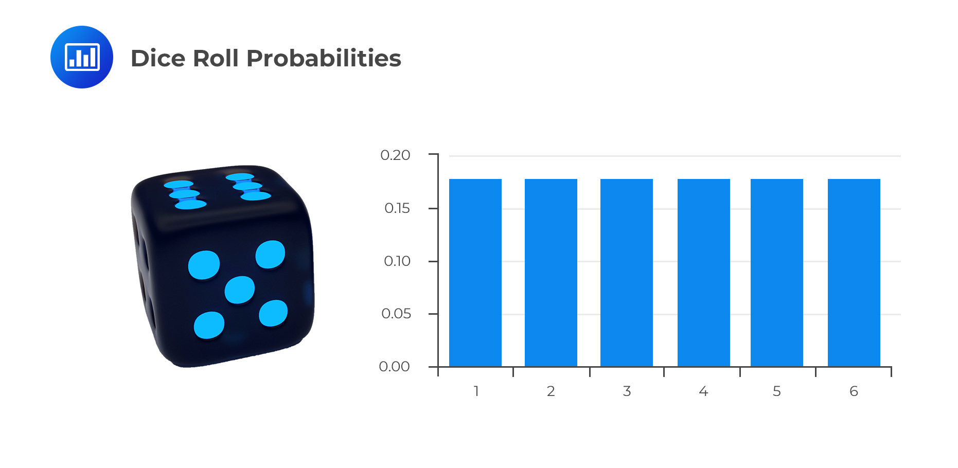
As you will recall, all possible outcomes have equal probabilities under the uniform distribution. A good example might be the throw of a die, where each outcome 1, 2, 3, 4, 5, and 6 has a 1/6 probability of occurrence.

Define the random variable \(\)X such that \(X_i=i\), where \(i = 1, 2, 3, …, k\)

$$ P(X = x) = \cfrac {1}{k} $$.

$$ \text{Mean} =\cfrac {(k + 1)}{2} $$.

$$ \text{Variance} = \cfrac {(k^2 – 1)}{12} $$.

Example: Uniform Distribution Function

A uniform distribution function has been defined as:

$$ X = \{1, 3, 5, 7, 9\} $$.

The value of \(P(X = 5)\) is closest to:

Solution

$$ \begin{align*} P(X = x) & = \cfrac {1}{k} \\ K & = 5\\ \end{align*} $$

Therefore,

$$ P(X = 5) =\cfrac {1}{5} = 0.2 $$

Question

A uniform distribution function has been defined as:

$$ X = \{1, 3, 5, 7, 9\} $$

The value of  \(F(5)\) is closest to:

1. 0.2.
2. 0.4.
3. 0.6.

Solution

The correct answer is C.

\(F(5)\) is the cumulative probability of an outcome less than or equal to 5. Therefore,

$$ \begin{align*} F(5) &=P(X\leq 5)\\& = P(X = 1) + P(X = 3) + P(X = 5) \\ & = 0.2 + 0.2 + 0.2 \\ & = 0.6 \\ \end{align*} $$