The Lognormal Distribution vs. the Normal Distribution

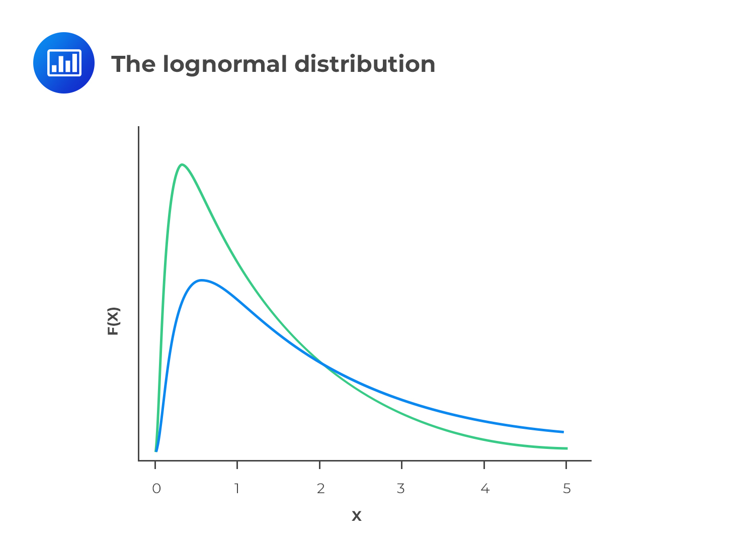
A variable X is said to have a lognormal distribution if Y = ln(X) is normally distributed, where “ln” denotes the natural logarithm. In other words, when the logarithms of values form a normal distribution, we say that the original values have a lognormal distribution.

Let’s consider this:

Y = e^x

If we take natural logs on both sides,

lnY = lne^x which leads us to lnY = x.

Therefore, if X has a normal distribution, then Y has a lognormal distribution with few large values. Consequently, the mean is greater than the mode in most cases.

Why the Lognormal Distribution is Used to Model Stock Prices

Since the lognormal distribution is bound by zero on the lower side, it is perfect for modeling asset prices that cannot take negative values. On the other hand, the normal distribution cannot be used for the same purpose because it has a negative side.

When the returns on a stock (continuously compounded) follow a normal distribution, the stock prices follow a lognormal distribution. Note that even if returns do not follow a normal distribution, the lognormal distribution is still the most appropriate model for stock prices.

The probability density function of the distribution is:

$$ f\left( x \right) =\frac { 1 }{ x\sqrt { 2\pi { \sigma }^{ 2 } } } { e }^{ -\frac { { \left( lnx-\mu \right) }^{ 2 } }{ \sqrt { 2{ \sigma }^{ 2 } } } } $$

The Black-Scholes model used in price options uses the lognormal distribution as its foundation.

Cheap stocks usually exhibit just a few large moves, and the price then stagnates. However, because the base is so low, even a very small price change translates to a large percentage change. For example, if the stock price is $2 and the price reduces by just $0.10, this translates to a 5% change. For this reason, while the stock return is normally distributed, price movements are best explained using a lognormal distribution.