


Methods of Solving Counting Problems
Counting problems involve determining the exact number of ways two or more operations... Read More

A contingency table is a tabular representation of category-based data. It shows the frequencies for particular combinations of values for two discrete random variables, say X and Y. Each cell in the table represents a mutually exclusive combination of X-Y values. A contingency table for two category-based variables is also known as a two-way table.
The following contingency table shows a hypothetical frequency distribution of women’s education level preference in three countries among a random sample of 120 females:
$$
\begin{array}{l|c|c|c|c}
\begin{array}{l}
\textbf { Education } \\
\textbf { level }
\end{array} & \textbf { Kenya } & \textbf { Uganda } & \textbf { Tanzania } & \textbf { Total } \\
\hline \begin{array}{l}
\text { Middle school } \\
\text { or lower }
\end{array} & 5 & 5 & 30 & 40 \\
\hline \text { High school } & 5 & 25 & 5 & 35 \\
\hline \text { Bachelor’s } & 15 & 5 & 5 & 25 \\
\hline \text { Master’s } & 15 & 5 & 0 & 20 \\
\hline \text { Total } & 40 & 40 & 40 & 120 \\
\end{array}
$$
The above table indicates that a ‘Middle school or lower level’ of education is dominant in Tanzania, while ‘High school’ is dominant in Uganda. Besides, according to the table, Kenyan women most often go up to a ‘Bachelor’s’ or ‘Master’s’ degree level. We can also see that no Tanzanian woman has a ‘Master’s’ degree within the sample.
Joint frequency is the number of times a combination of two conditions happens together. For example, ‘Kenya’ and ‘Middle school or lower’ have a joint frequency of 5.
The sum of the joint frequencies across rows and columns is called marginal frequencies. For example, the marginal frequency of ‘Bachelor’s’ degree is the sum of the joint frequencies across all three countries, that is, 25 (= 15 + 5 + 5). ‘Middle school or lower’ and ‘High school’ have the largest marginal frequencies.
We can also create contingency tables by using relative frequencies. For example, the preference for ‘High school’ in Uganda is \(\frac{25}{120} = 21\%\).
$$\begin{aligned} &\textbf{Relative Frequency as % of total}\\
&\begin{array}{l|c|c|c|c}
\begin{array}{l}
\textbf { Education } \\
\textbf { Level }
\end{array} & \textbf { Kenya } & \textbf { Uganda } & \textbf { Tanzania } & \textbf { Total } \\
\hline \begin{array}{l}
\text { Middle school or } \\
\text { lower }
\end{array} & 4 \% & 4 \% & 25 \% & \mathbf{3 3} \% \\
\hline \text { High school } & 4 \% & 21 \% & 4 \% & \mathbf{2 9} \% \\
\hline \text { Bachelor’s } & 13 \% & 4 \% & 4 \% & \mathbf{2 1} \% \\
\hline \text { Master’s } & 13 \% & 4 \% & 0 \% & \mathbf{1 7} \% \\
\hline \textbf { Total } & \mathbf{3 3 \%} & \mathbf{3 3} \% & \mathbf{3 3 \%} & \mathbf{1 0 0} \% \\
\end{array} \end{aligned}$$
$$\begin{aligned}&\textbf{Relative Frequency: Frequency Distribution in the Region as % of}\\&\textbf{Total Frequency (Preference)}\\
&\begin{array}{l|c|c|c|c}
\textbf { Education Level } & \textbf { Kenya } & \textbf { Uganda } & \textbf { Tanzania } & \textbf { Total } \\
\hline \text { Middle school or lower } & 13 \% & 13 \% & 75 \% & \mathbf{3 3} \% \\
\hline \text { High school } & 13 \% & 63 \% & 13 \% & \mathbf{2 9} \% \\
\hline \text { Bachelor’s } & 38 \% & 13 \% & 13 \% & \mathbf{2 1} \% \\
\hline \text { Master’s } & 38 \% & 13 \% & 0 \% & \mathbf{1 7} \% \\
\hline \textbf { Total } & \mathbf{1 0 0} \% & \mathbf{1 0 0} \% & \mathbf{1 0 0} \% & \mathbf{1 0 0} \% \\
\end{array}\end{aligned}
$$
A confusion matrix is a summary of prediction results on a classification problem. The number of correct and incorrect predictions is summarized with count values and broken down by each class. A confusion matrix is one of the applications of a contingency table.
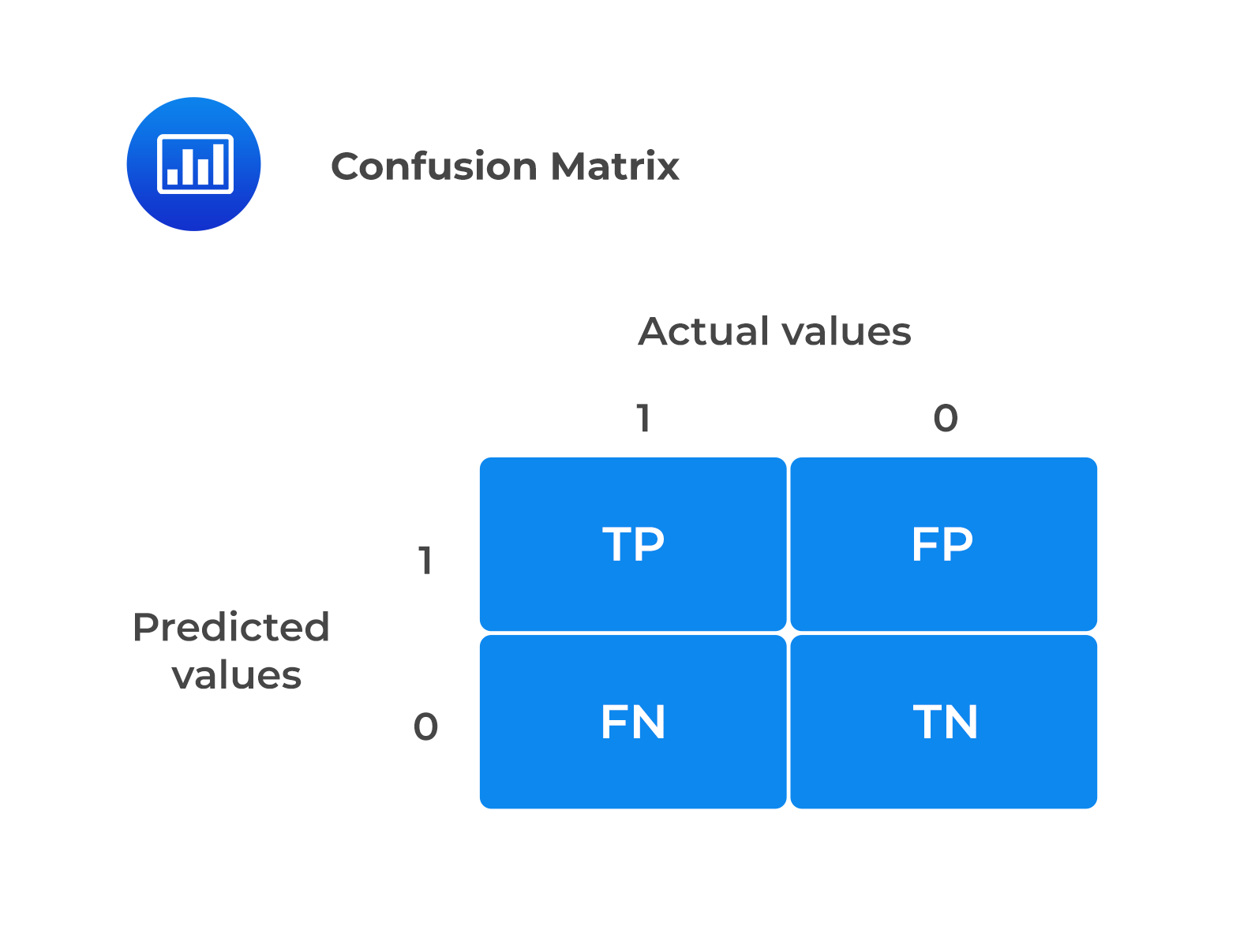
A confusion matrix represents different combinations of actual versus predicted values.
Let us consider the example of a stock market negative return prediction using a confusion matrix. Assume that we have 1000 records in our dataset regarding the stock market return of negative 20% or more. Refer to the following confusion matrix:
$$
\begin{array}{ll|ll|l}
& & \textbf { Stock Market negative } & & \\
& & \textbf { return of 20 % or more } & & \\
& & \textbf { Actual values } & & \\
& & & & \\
& & \text { YES } & \text { NO } & \textbf { Total } \\\hline
\textbf { Stock Market Negative } & \text { YES } & 460 & 200 & 660 \\
\textbf { Return of 20% or more } & & & & \\
\textbf { Predicted Values } & \text { NO } & 150 & 190 & 340 \\
\end{array}
$$
In the above matrix, we can make the following deductions:
A contingency table can also be used to investigate the potential association between two category-based variables. We can test the association between category-based variables by performing a chi-square test of independence. This involves the following steps:
The following example describes how a contingency table is used to set up this test of independence.
Example: Contingency Tables and Association between Two Categorical Variables
We have 200 bonds, and we can classify them in two ways: by issuer, either a corporate or a financial institution, and by risk level, either low risk or high risk. The data are summarized in a 2 × 2 contingency table shown below.
$$
\begin{array}{l|c|c}
\textbf { Contingency Table } & & \\
\hline & \textbf { Low Risk } & \textbf { High Risk } \\
\hline \textbf { Bonds issued by a Corporation } & 27 & 57 \\
\hline \begin{array}{l}
\textbf { Bonds issued by a Financial } \\
\textbf { Institution }
\end{array} & 95 & 21 \\
\end{array}
$$
Questions
The Solution to Question 1
The task is to calculate the marginal frequencies based on the type of issuer. To do this, we must add joint frequencies across the rows. Therefore, the marginal frequency for corporations is 27 + 57 = 84, and the marginal frequency for financial institutions is 95 +21 = 116.
The Solution to Question 2
The task is to calculate the marginal frequencies based on the bond’s risk. We do this by adding joint frequencies down the columns. Therefore, the marginal frequency for low risk is 27 + 95 = 122, and the marginal frequency for high risk is 57 + 21 = 78.
The Solution to Question 3
Based on the procedure for conducting a chi-square test of independence, we would perform the following three steps:
Step 1: Add the marginal frequencies and overall total to the contingency table. We have also included the relative frequency table for observed values.
$$
\begin{array}{l|c|c|c|l|c|c|c}
& \textbf { Low Risk } & \textbf { High Risk } & & & \begin{array}{c}
\textbf { Low } \\
\textbf { Risk }
\end{array} & \begin{array}{c}
\textbf { High } \\
\textbf { Risk }
\end{array} & \\
\hline \begin{array}{l}
\text { Bonds issued by } \\
\text { Corporations }
\end{array} & 27 & 57 & 84 & \begin{array}{l}
\text { Bonds issued } \\
\text { by Corporations }
\end{array} & 32 \% & 68 \% & 100 \% \\
\hline \begin{array}{l}
\text { Bonds issued by } \\
\text { Financial } \\
\text { Institutions }
\end{array} & 95 & 21 & 116 & \begin{array}{l}
\text { Bonds issued } \\
\text { by Financial } \\
\text { Institutions }
\end{array} & 82 \% & 18 \% & 100 \% \\
\hline & 122 & 78 & 200 & & & & \\
\end{array}
$$
Step 2: Use the marginal frequencies in the contingency table to construct a table with the expected values of the observations. To determine the expected values for each cell, multiply the respective row total by the respective column total, then divide by the overall total. So, for cell i,j (in ith row and jth column):
$$\text{Expected Value}_{i,j} = \frac{\text{Total Row i × Total Column j}}{\text{Overall Total}}$$
For example,
The expected value for corporate bonds or low risk is:
$$\frac{84 × 122}{ 200} = 51.24$$
And expected value for financial institutions or high risk is:
$$ \frac{116 × 78}{200} = 45.24.$$
The table of expected values (and accompanying relative frequency table) would look like this:
$$
\begin{array}{l|c|c|c|l|c|c|c}
& \begin{array}{l}
\textbf { Low } \\
\textbf { Risk }
\end{array} & \begin{array}{l}
\textbf { High } \\
\textbf { Risk }
\end{array} & & & \begin{array}{l}
\textbf { Low } \\
\textbf { Risk }
\end{array} & \begin{array}{c}
\textbf { High } \\
\textbf { Risk }
\end{array} & \\
\hline \text { Bonds issued by Corporations } & 51.2 & 32.8 & 84 & \begin{array}{l}
\text { Bonds } \\
\text { issued by } \\
\text { Corporations }
\end{array} & 61 \% & 39 \% & 100 \% \\
\hline \begin{array}{l}
\text { Bonds issued by Financial } \\
\text { Institutions }
\end{array} & 70.8 & 45.2 & 116 & \begin{array}{l}
\text { Bonds } \\
\text { issued by } \\
\text { Financial } \\
\text { Institutions }
\end{array} & 61 \% & 39 \% & 100 \% \\
\end{array}
$$
Step 3: Derive the chi-square test statistic and then compare it to a value from the chi-square distribution for a given level of significance.
Question
The following contingency table shows the frequency of consumption of three common brands of bread in three geographic regions among a random sample of 100 consumers:
$$
\begin{array}{l|c|c|c}
\textbf { Brands } & \textbf { Region 1 } & \textbf { Region 2 } & \textbf { Region 3 } \\
\hline \mathrm{A} & 5 & 5 & 30 \\
\hline \mathrm{B} & 5 & 25 & 5 \\
\hline \mathrm{C} & 15 & 5 & 5 \\
\end{array}
$$Which brand most likely has the highest marginal frequency?
- Brand A.
- Brand B.
- Brand C.
Solution
The correct answer is A.
Note that the marginal frequency of a contingency table is the sum of the joint frequencies across rows and columns. In this case, we are dealing with the rows (Bread brands). Based on the calculation below, Brand A has the highest marginal frequency.
$$
\begin{array}{l|c|c|c|c}
\textbf { Brands } & \textbf { Region 1 } & \textbf { Region 2 } & \textbf { Region 3 } & \textbf { Total } \\
\hline \mathrm{A} & 5 & 5 & 30 & 40 \\
\hline \mathrm{B} & 5 & 25 & 5 & 35 \\
\hline \mathrm{C} & 15 & 5 & 5 & 25 \\
\end{array}
$$
Strengthen your understanding of probability relationships, independence testing, and data interpretation with structured CFA Level I practice.


Get Ahead on Your Study Prep This Cyber Monday! Save 35% on all CFA® and FRM® Unlimited Packages. Use code CYBERMONDAY at checkout. Offer ends Dec 1st.