Fixed Income – Level I CFA® Exam Essential Review Summary – offered by AnalystPrep

Reading 42 – Fixed-Income Securities: Defining Elements

A bond is a debt instrument that entitles the buyer to future cash flows from the issuing entity. Bonds can be issued by a variety of organizations, including companies, governments, and even supranational groups like the European Union. Bonds are categorized into three primary sectors based on issuer and structure: Government, Corporate, and Structured Finance. Bonds are also categorized by the level of credit risk they have. Higher-quality bonds are known as Investment Grade and have lower yields, while riskier bonds (more likely to default) are known as High-Yield (sometimes referred to as “junk bonds”).

A traditional bond is a promise to pay back a borrowed amount (the “par” value of the bond) plus interest over a specified time period. This typically involves periodic payments of the interest and then a final repayment of the original principal amount at the maturity date.

The legal document that specifies all the parameters of a particular bond is the Indenture. It will describe all the important information such as the issuer, par amount, coupon rate and frequency, and any covenants. The covenants are rules specific to that bond issue that the borrowers and lenders agree to at the time of the bond issuance. The indenture will also outline whether the bond is secured or unsecured and what assets are backing the bond if it is secured. Bonds can also contain credit enhancements to help decrease the credit risk, such as insurance against default, overcollateralization, or even reserve accounts that can be drawn against to make payments.

Bonds are subject to numerous legal and regulatory requirements, and one categorization that determines how they are regulated is the domicile of the issuer in relation to where the issue takes place. If an entity issues a bond in their own country, it is considered a Domestic Bond. If an entity issues a bond in a different country, it is considered a Foreign Bond.

The most common structure for a bond involves periodic fixed interest payments and a lump sum of the principal at the maturity date. These periodic interest payments are known as coupon payments. There are also bonds that are amortizing, which means that each periodic payment includes both interest and repayment of part of the principal amount. The coupon rates for bonds can be either fixed or floating, which means that the interest payments will either remain consistent over time or change in relation to a specified benchmark rate.

Bonds can include contingencies that provide additional rights to the issuer and/or the bondholders. One of these is a call option. Callable Bonds give the issuer the right to redeem (call) the bond by repaying the principal amount before the bond reaches maturity. This is useful for issuers when interest rates drop, and they are able to repay an older bond with higher interest with funds from a new issue at the lower rates. Puttable Bonds give the bondholders the right to sell (put) the bond back to the issuer. Bondholders may want to exercise this option if rates have increased, and they want to sell that bond and purchase newer bonds with higher yields. Convertible Bonds are a hybrid of debt and equity securities. These give the right to convert the bonds into equity shares in the company in certain situations.

Reading 43 – Fixed-Income Markets: Issuance, Trading and Funding

As mentioned in the previous section, floating rates bonds differ from their fixed rate counterparts in that the coupon rate changes over time-based on movements of a specified reference rate. The most commonly used reference rate is the London InterBank Offered Rate (LIBOR).

Similar to equity securities, there are both primary markets (where new bonds are sold to investors for the first time) and secondary markets (where existing bonds are bought and sold between investors) for bond securities. There are a number of mechanisms by which new bonds are issued in primary markets. In an Underwritten Offering, an investment bank guarantees the sale of new bonds at a negotiated offering price. The investment bank takes on the risk of this price guarantee because they are responsible for buying any remaining bonds that they are unable to sell at that price. For larger bond offerings, multiple underwriters may work together in what is known as a Syndicated Offering. Some issuers use the Shelf Registration approach, wherein they get approval for a new offering that may not take place right away. They retain the ability to issue new bonds as part of that offering in the near future without going through a new registration.

Secondary trading for bonds can take place either on an exchange or over-the-counter (OTC). On an exchange, trade orders are submitted to the exchange and matched with other orders based on exchange criteria, similar to what one sees on an electronic stock exchange. In OTC trading, buyers and sellers contact each other directly to negotiate trades. The vast majority of bond trading is done via OTC.

The difference between the bid and ask quotes in the market for a specific bond (the bid-ask spread) is an indicator of the liquidity for that security. The larger the spread, the less liquid that bond likely is. Compared to equity securities, individual bonds trade much less frequently and tend to have commensurately larger spreads. When bonds do trade, they typically settle on either a T+1 basis (for government bonds) or a T+2 or T+3 basis (for corporate bonds).

US government bonds are denoted differently depending on their time to maturity. Issues made with less than 1 year to original maturity are known as T-bills, while T-notes and T-bonds have longer maturities. T-bills are issued as discount notes, meaning that they are issued at a price less than par. T-notes and T-bonds are more typical bonds that are issued at par.

In addition to traditional corporate or government bonds, there are also several categories of bonds issued in conjunction with governments but are not considered government bonds. Non-sovereign bonds are those issued to help fund public projects but are not guaranteed by national governments. They typically have low default rates but have higher yields than guaranteed government bonds. There are also quasi-government bonds that are also not guaranteed but often have an implied government backing. Examples of issuers of these bonds are the semi-government organizations Fannie Mae and Freddie Mac. There are even bonds issued by agencies that exist in multiple countries which are known as supranational bonds. Organizations like the IMF and European Union issue bonds outside of any individual nation.

Companies issue debt as a way to get funding for investments in their operations. When companies need short-term funding, they can issue Commercial Paper, which consists of debt with maturities generally less than 3 months and as short as overnight. The commercial paper market is extremely liquid, as companies frequently pay off loans with funding from new short-term issuances (this is known as “rolling” the debt).

Banks have additional sources of short-term funding available to them, such as Interbank Lending and Central Banks, where they can borrow or loan money with other banks for terms of less than 1 year. One source of funding for banks are Certificates of Deposit, wherein they offer higher rates to depositors in exchange for having a fixed period before the deposits can be withdrawn.

A special type of lending facility is the Repurchase Agreement, also known as a repo. These consist of the sale of a security (usually financial market securities) and an agreement to buy back the security at a specified future date at an agreed-upon price. These are naturally collateralized because the asset involved in the repo agreement serves as collateral for the loan.

Reading 44 – Introduction to Fixed-Income Valuation

Similar to equity securities, the price of a bond should be the present value of the expected future cash flows. Unlike equity securities, these cash flows tend to be finite and known in advance. Especially for plain vanilla coupon bonds, the buyer will know the exact amounts and dates of the cash flows they will receive. This means that it is relatively straightforward to calculate the present value of those cash flows, discounted using the current market interest rate. Since the market rate serves as the discount rate, we expect the price of a bond to decrease as rates increase, since it means we are more heavily discounting the cash flows. Intuitively, this should also make sense because a bond whose coupon rate is below the new market rate should be worth less than it was before since the investor could now sell that bond and buy another one with a higher coupon.

Similar to equity securities, the price of a bond should be the present value of the expected future cash flows. Unlike equity securities, these cash flows tend to be finite and known in advance. Especially for plain vanilla coupon bonds, the buyer will know the exact amounts and dates of the cash flows they will receive. This means that it is relatively straightforward to calculate the present value of those cash flows, discounted using the current market interest rate.

The general formulae for calculating the present value of a bond is as shown below:

$$ {PV}_{bond}=\frac{PMT}{({1+i)}^1}+\frac{PMT}{{(1+i)}^2}+\ldots+\frac{PMT}{{(1+i)}^n} $$

Where:

PMT is the Coupon Payment Per Period

FV  is the Face Value of the bond at maturity

i is the Market Discount Rate

For example, the calculation of the price for a 5-year bond that pays a 5% coupon annually when the market rate is 6% would be as follows:

$$
\begin{array}{l|cccccc}
\text{Time Period} & 1 & 2 & 3 & 4 & 5 \\
\hline
\text{Calculation} & \frac { \$5 }{ { \left( 1+6\% \right) }^{ 1 } } & \frac { \$5 }{ { \left( 1+6\% \right) }^{ 2 } } & \frac { \$5 }{ { \left( 1+6\% \right) }^{ 3 } } &a \frac { \$5 }{ { \left( 1+6\% \right) }^{ 4 } } & \frac { \$105 }{ { \left( 1+6\% \right) }^{ 5 } } \\
\hline
\text{Cash Flow} & \$4.717 & +\$4.450 & +\$4.198 & +\$3.960 & +\$78.462 & =\$95.788 \\
\end{array}
$$

This bond would be trading at less than its par value of 100 (known as a discount) because it’s current rate is less than what’s available in the market. If the bond’s coupon rate were higher than the market rate, we would expect it to be trading at a premium to its par value.

Since the market rate serves as the discount rate, we expect the price of a bond to decrease as rates increase, since it means we are more heavily discounting the cash flows. Intuitively, this should also make sense because a bond whose coupon rate is below the new market rate should be worth less than it was before since the investor could now sell that bond and buy another one with a higher coupon.

You will likely be asked to calculate the Yield to Maturity for a bond security, which is the internal rate of return that sets the present value of the future cash flows equal to the current price. You will use the time value of money functionality on your calculator to solve for this value the same way that you solved for IRR values in the Quantitative Methods section. The only change you may see that might not have occurred in that section is to change the “P/Y” value, because most common bonds make two interest payments per year. You change this value on your calculator the way you change any other time value, by pressing 2 and then the P/Y button. Be sure to keep track of what you have this value set to because you will definitely see questions involving bonds with varying numbers of payments per year. The curriculum refers to this annual frequency of payments as the Periodicity.

It is also important to note that the price of a bond moves closer to the par value as the maturity of the bond nears. Also, the prices of longer-term bonds vary more than those of shorter-term bonds.

In addition to finding the Yield to Maturity for a given bond, you can also find its current price using spot rates. This is a similar calculation except that you will use different discount rates for each cash flow that you are discounting. Rather than using the time value of money functionality on your calculator for these problems, you’ll manually calculate the present value of each cash flow using the spot rate given for that time period, as per the below formula:

$$ {PV}_{bond}=\frac{PMT}{{(1+Z_1)}^1}+\frac{PMT}{{(1+Z_2)}^2}+\ldots+\frac{PMT+Principal}{{(1+Z_n)}^n} $$

Bond prices can be quoted in two different ways due to the nature of their interest accruals. The Flat Price of the bond is calculated the way we’ve covered up until now.

The Full Price (also called the “dirty price”) includes the Flat Price and the interest that has accrued since the last interest payment, \({PV}^{full}={PV}^{flat}+\text{Accrued Interest}\). If given the market discount rate per period (r), the full price can be calculated using the formula \({PV}^{full}=PV\times{(1+r)}^{t/T}\), where \({t/T}\) is the proportion of the coupon period that has passed since the last payment.

The Accrued Interest is the proportional share of the upcoming interest payment. This is included in the Full Price so that the investor selling the bond doesn’t lose out on the amount of interest they would have received for the part of the accrual period in which they owned the bond. The accrued interest is calculated by taking the next coupon payment and multiplying it by the percentage of the coupon period that has passed since the last payment:

$$ \text{Accrued Interest}=\frac{t}{T}\times PMT $$

When calculating this elapsed time, it’s important to know the day-count methodology being used. There are 2 primary methods used for this: Actual-actual and 30/360. In the 30/360 method, each month is assumed to have 30 days and a year is assumed to have 360 days. In the actual-actual method, the exact number of calendar days that are in each month and year are used.

As mentioned earlier, bonds do not trade as frequently as equities so it is more often necessary to calculate the correct current price for them. One method is to estimate the market discount rate and price based on the quoted or traded prices of similar securities that have recently traded. This method is known as Matrix Pricing. It utilizes the market prices of securities with similar maturities, credit quality, and other characteristics to calculate a price for a given security that may not have traded. Since matrix pricing using many securities is computationally intensive, you will likely only be asked to use a few securities in a question on this topic. For example, with quantitative factors like maturity, you can find the appropriate yield to maturity for a bond by finding the average of the yields to maturity for securities with a longer and shorter maturity.

In order to compare the yields of bonds with different payment frequencies, bond yields are typically annualized. This is the same calculation principle from the Quantitative Methods section. When you use the time value of money functionality on your calculator to find the yield to maturity, that value is already annualized. You will likely be asked to compare the yields for bonds that have similar characteristics but different periodicities.

The Periodicity of a rate of r% compounded semi-annually is 2. To get the annual rate for a periodicity of 2, we take r%×2. The periodicity of a rate of r% compounded quarterly is 4. To get the annual rate for a periodicity of 4, we take r%×4, and so on and so forth. To convert rates between different periodicities, we use the general formula:

$$( 1+\frac{APR_m}{m})^m= (1+\frac{APR_n}{n})^n $$

$$ \text{Where } m \text{ and } n \text{are the different periods within a year} $$

When valuing bonds, it is important to consider that bonds can either be Fixed-Rate Bonds (pay the same amount of interest for a specified term) or Floating-Rate Bonds (interests vary depending on the level of the reference interest rate).

Fixed rate bonds can be valued using: Street Convention (assumes that payments are made on scheduled dates excluding weekends and holidays), True-Yield (IRR calculated using a calendar and includes weekends and holidays), Current Yield (calculated as the sum of  the bond’s coupon payments over one year divided by the flat price of the bond) or Simple Yield (calculated as the sum of the coupon payments and straight-line proportion of the gain or loss, divided by the flat price of the bond.)

For money markets instruments, bond yields to maturity are annualized but not compounded, and are quoted using non-standard rates (discount rates and add on rates).

$$ PV=FV\times(1-\frac{\text{Number of days between settlement and maturity}}{\text{Number of days in a year}}\times\text{Annualized discount rate}) $$

When using the discount rates to price money market instruments,

$$ \text{Annualized discount rate}=(\frac{\text{Number of days in a year}}{\text{Number of days between settlement and maturity}})\times(\frac{FV-PV}{PV}) $$

When using add on rates,

$$ PV=(\frac{FV}{1+\frac{\text{Number of days between settlement and maturity}}{\text{Number of days in a year}}\times \text{Annualized add­ on rate}}) $$

To calculate the Annualized add­ on rate,

$$ AOR=(\frac{\text{Number of days in a year}}{\text{Number of days between settlement and maturity}})\times(\frac{FV-PV}{PV}) $$

To compare the yields of money market instruments on the same basis, we have to use the bond equivalent yield. The bond equivalent yield is quoted on a 365-day add-on rate basis and is obtained by converting one rate to another.

A graph of all of the yields for a type of security along the range of maturities is known as a Yield Curve. Yield curves are upward sloping because longer-maturity bonds have higher yields, but the slope flattens out at longer maturities because the yield differences become much smaller for each additional time to maturity at the long end. This version of the yield curve is known as the Spot Curve because it shows the spot rate for each maturity period. There is also a Par Curve which is the same except it shows the yield-to-maturity for bonds priced at par at each point in the maturity curve. Par curves are calculated based on spot curves and represent the difference in yields due to changes in maturity but holding every other bond characteristic the same.

Bond rates can be quoted in terms of spot rates or forward rates, depending on whether the bond funding is being provided right now or at some point in the future. A spot rate applies when the bond is to be issued now and the rate will apply immediately, while the forward rate is used when the bond will be issued in the future. Implied forward rates are calculated based on spot rates. The implied forward rate is the rate that sets the current spot rate and the spot rate for the period covering both the current spot and forward periods equal. For example, the implied forward rate for a 3-year bond to be issued 2 years in the future would be calculated as follows:

$$ { \left( 1+{ r }_{ 2 } \right) }^{ 2 }\ast { \left( 1+{ IFR }_{ 2,3 } \right) }^{ 3 }={ \left( 1+{ r }_{ 5 } \right) }^{ 5 } $$
$$ { r }_{ 2 }=2-year\quad spot\quad rate $$
$$ { r }_{ 5 }=5-year\quad spot\quad rate $$
$$ { IFR }_{ 2,3 } = Implied\quad Forward\quad Rate $$

You can also create a curve of these forward rates extending along the maturity dates and this would be known as the Forward Curve.

Yield spread is the difference between any two bond issues. There are 4 types of spreads:

1. G-Spread is the difference between the yield on the corporate bond and the yield on a government bond.
2. I-Spread is the difference between the yield on a bond and the swap rate.
3. Z-Spread is the constant spread that makes the price of a security equal to the present value of its cash flows when added to the yield at each point on the spot rate Treasury curve.
4. Option-Adjusted Spread (OAS) is the difference between the Z-spread and the option value.

Reading 45 – Introduction to Asset-Backed Securities

Asset-Backed Fixed Income Securities (ABS) are different than the bonds already covered here because, rather than being based on an amount lent to an issuer that they pay back over time, they are based on pools of assets that are securitized and combined into one fixed income security. The pool of assets from which the security’s cash flows derive is known as its collateral. These are very common for mortgages and other consumer lending products since it allows these (relatively) smaller loan amounts to be bundled together to create fixed income assets large enough to be purchased by institutional investors.

The pools of assets that underly an asset-backed security are held in legal ownership by an entity created just for that purpose rather than owned by the issuer. These entities (known as Special Purpose Entities, or SPEs) control the assets, receive the cash flows from the individual borrowers (for example, mortgagees), and distribute these cash flows to the bondholders. The SPEs can sometimes use another organization as the servicer, in which case that servicer is the one that receives and distributes the cash flows even though the SPE maintains the ownership of the assets.

ABS can be divided up into multiple classes of bonds based on characteristics like credit and default risk. The more subordinated (lower in rank) a class is, the higher the coupon payments but also the higher the default risk. These classes typically function in a waterfall structure, where the cash flow distributions are made in order of class, starting with the most senior, and the default losses are assessed in the reverse order. Investors can choose the level of risk and yield they wish to expose themselves to by purchasing at different class levels.

One common source of assets for ABS bonds are mortgage loans. These are categorized as either prime or sub-prime depending on how creditworthy the borrowers and how risky the loans are. An important risk to consider in mortgage ABS is that of prepayment risk. Since many mortgage borrowers are able to pay their mortgages off early or refinance when rates go down, there is an increased risk that the ABS will lose assets early and the investor will have to reinvest that money into newer, lower yielding securities. A potentially more costly risk regarding mortgages is borrowers defaulting and the properties being foreclosed upon. The ABS investor is entitled to proceeds from foreclosure sales but there is often a shortfall between those proceeds and the original value of the mortgage loan.

Mortgages are categorized by whether they are Agency or non-Agency. Agency mortgages are those guaranteed by a federal agency or a government-sponsored entity like Fannie Mae. Non-agency mortgages are those that do not have any of these guarantees and are issued by private entities, so these mortgages generally carry higher yields and represent a higher credit risk to the investor.

Since the rates of prepayment for mortgage ABS (MBS) will impact how long it takes for the security to mature (because the security matures when all underlying mortgages are paid off), there are risks to track that don’t apply to all bond securities. If rates go down, there is a risk of maturity contraction because mortgage borrowers can refinance their loans at lower rates, which pays off the original loans early. The opposite risk is that of extension, where the mortgage security takes longer to fully mature because rates go up and mortgage borrowers prepay more slowly.

One measure of this is the Single Monthly Mortality Rate (SMM), which represents the monthly repayment of the mortgage pool. It is the prepayments for a specific month divided by the outstanding mortgage pool balance. This rate can also be annualized, which is known as the Conditional Prepayment Rate (CPR).

Another source of funding for ABS is from commercial property mortgages. These are known as Commercial Mortgage-Backed Securities (CMBS). The credit risk of these securities is quantified using the loan-to-value ratio (LTV) and the debt-service-coverage (DSC). The higher these values are, the more credit risk these loans represent. Commercial mortgage loans are more likely to have prepayment penalties, so the prepayment risk is less than what it is for MBS bonds. There are several other common sources for funding in ABS bonds. There are securities based on auto loans, auto lease receivables, and credit card receivables (somewhat riskier because these are unsecured loans).

Collateralized Debt Obligations (CDO) are securities backed by a diversified pool of one or more debt obligations. They can be backed by corporate bonds, ABS, or even other CDOs. These are usually structured in several tranches that represent different levels of credit risk and seniority in receiving cash flows. These involve the creation of SPEs who own the underlying assets and exist only as a vehicle for managing the pool of assets until the CDO matures. The riskiest tranche of a CDO is known as the equity tranche and is the first class to be impacted by defaults in the pool of assets.

Reading 46 – Understanding Fixed-Income Risk and Return

The return from a fixed-income security can be broken down into three sources: the coupon and principal payments received, reinvestment of the coupon payments, and capital gains (or losses) on the sale of the bond before maturity. Bonds that trade at a premium or discount to par value will amortize to par as the bond approaches maturity.

The calculation for returns on reinvested coupons involves finding the future value of the coupon payments using the yield to maturity of the bond. You can use the time value of money functions on your calculator using the coupons as the PMT amount and the yield to maturity as the I/Y value to find the total return from reinvestment. The amount of this future value in excess of the coupons themselves is known as the “interest-on-interest” gain from compounding. The internal rate of return between the total return (the sale price plus the sum of coupons and interest-on-interest gains) and the original purchase price is known as the horizon yield.

Bond Duration is the measurement of a bond’s full price to changes in interest rates and is a very important part of the fixed income curriculum. There are two types of duration: yield duration is the sensitivity of a bond’s price to changes in its own yield-to-maturity (discount rate) and curve duration measure the sensitivity to changes in a specified benchmark rate (usually government rate curves).

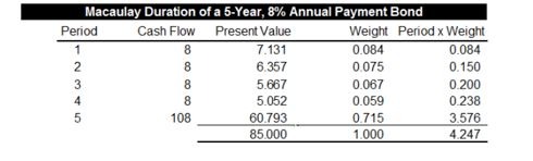
There are several duration calculations that are used in the curriculum. Macaulay Duration is the weighted average of the present values of all future cash flows for a bond. The table below outlines the calculation of the Macaulay duration for a traditional bond. In this example, the present values were found using the bond’s yield to maturity of 12.18%. The weight column is each cash flow as a percentage of the total present value (the 85 at the bottom of column 3). Once the present values are multiplied by their weights (column 5), the sum of those values (4.247) represents the Macaulay duration for the bond:

Modified Duration is based on the Macaulay duration. The formula for it is:

$$ Modified\quad Duration=\frac { Macaulay\quad Duration }{ 1+YTM } $$

The Effective Duration is the sensitivity of a bond’s total price to changes in a specified benchmark rate (usually a government yield curve)

$$ Effective\quad Duration=\frac { { PV }_{ – }-{ PV }_{ + } }{ 2\ast \left( \Delta Curve \right) \ast { PV }_{ 0 } } $$
$$ { PV }_{ – }=new\quad PV\quad when\quad curve\quad is\quad raised $$
$$ { PV }_{ + }=new\quad PV\quad when\quad curve\quad is\quad lowered $$
$$ { PV }_{ 0 }=original\quad PV\quad of\quad bond $$
$$ \Delta Curve=curve\quad change $$

Effective duration is especially useful for securities with call or other options. Since the likelihood of exercising a call or put option varies with changes in interest rates, it is important to know how sensitive they are to these rate changes. Because there is more uncertainty regarding their future cash flows, it is also hard to define a consistent yield-to-maturity for these bonds and therefore harder to calculate a useful Macaulay or Modified duration figure.

Key Rate Durations measure a bond’s sensitivity to changes in benchmark yield curves at specific points of maturity. Whereas the effective duration is based on parallel shifts of the entire yield curve, key rate durations break down that exposure to sections of the curve.

The measures of duration (which are expressed in years) will always be less than the time to maturity for a typical coupon bond. The Maturity Effect states that a longer-term bond is more sensitive to interest rate changes than a shorter-term bond. Longer maturity bonds will tend to also have higher duration values. Since Macaulay and Modified duration is based on the yield-to-maturity as the discount factor, higher yielding bonds will have lower duration values than ones with lower yields. Since bonds with put options can be sold when rates rise, their effective duration will be lower than bonds without similar protections for the investor.

Similarly to the way in which duration is used for individual bond securities, the duration of a portfolio of fixed income securities is an important risk metric. The most accurate way to calculate the duration of a fixed income portfolio would be to find the weighted average of all cash flows for all bonds in the portfolio. Since this is computationally intensive, the more common approach is to find the weighted average of the durations of all bonds in the portfolio. This gives the Macaulay duration of the portfolio as a whole and the Modified duration can be found using the normal formula.

The modified duration tells you the expected percentage change of a bond’s price given a change in its yield to maturity. Another way this can be expressed is to calculate the Money Duration (also known as dollar duration). This value is simply the annual modified duration multiplied by the Full Price of the bond. The new value will tell you the actual dollar amount of value change to be expected for a change in yield to maturity. A similar measure is the Price Value of a Basis Point, which is calculated by taking the difference between the prices of a bond given a 1bp increase and a 1bp decrease in yield to maturity and dividing that value by 2. This is the value, in dollars, attributed to a single basis point of yield to maturity. The calculation uses the average for both an increase and a decrease in yield because convexity means the increase and decrease could cause different changes in price. Remember that one basis point is equivalent to 0.01% (1/100th of a percent) or 0.0001 in decimal.

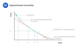
The Convexity Effect describes how a bond’s price will change in relation to interest rate changes. It directs that the percentage price change is greater for rate decreases than rate increases.

The Convexity Effect shows up in graphical form when looking at how the price of a bond continues changing as rates continue to change. Rather than following a straight line, the convexity of a bond describes how the bond can become more or less sensitive to each additional change in interest rates. In the graph below, Bond A is demonstrating strong convexity and the amount by which its price change varies along the line of possible interest rates.

Convexity can either be Approximate Convexity or Effective Convexity. Approximate convexity is used to improve the estimate of the percentage price change:

A convexity measure is used to improve the estimate of the percentage price change.

$$ \text{Change in price of a bond} = \text{Duration effect} + \text{Convexity effect} $$

$$\%ΔPV^{FULL}≈(\text{-AnnModDur}×ΔYield)+(\frac{1}{2}×\text{AnnConvexity}×(ΔYield)^2)$$

Effective convexity measures the secondary effect of a change in a benchmark yield curve:

$$ Approximate\quad Convexity=\frac { { PV }_{ – }+{ PV }_{ + }-\left( 2\ast { PV }_{ 0 } \right) }{ { \left( \Delta Yield \right) }^{ 2 }\ast { PV }_{ 0 } } $$
$$ { PV }_{ – }=new\quad PV\quad when\quad yield\quad declines $$
$$ { PV }_{ + }=new\quad PV\quad when\quad yield\quad increases $$
$$ { PV }_{ 0 }=original\quad PV\quad of\quad bond $$
$$ \Delta Yield=yield\quad change $$

The main difference between approximate and effective convexity is that approximate convexity is based on a yield to maturity change, whereas effective convexity is based on a benchmark yield change.

Interest rate changes greatly affect the prices of fixed income securities. To measure and manage the risk arising from interest rate shifts, analysts use duration to establish the sensitivity of a portfolio to changes in the level of interest rate changes. Interest rate increases with an increase in expected yield volatility.

A long term investor is majorly concerned with total return over the investment horizon. A buy-and-hold investor has a higher total return if interest rates rise and a lower total return if rates fall. Duration measures the immediate drop in value or price of interest rates. The bond is, however, “pulled to par” as time passes. At some point in the lifetime of the bond, those two effects offset each other, and the gain on reinvested coupons is equal to the loss on the sale of the bond. That point is the Macaulay Duration statistic. The difference between the Macaulay duration and the investment horizon is known as the Duration Gap. An investor is hedged against interest rate risk when the duration gap is zero, exposed to lower interest rate risk when the duration gap is negative, and to higher interest rate risk when it is positive.

The yield to maturity of a corporate bond is dependant on a government benchmark yield and a spread over that yield. The benchmark yield changes with a change in the expected inflation rate/expected real interest rate. The spread over the yield changes with changes in Credit Risk of the issuer and Liquidity of the bond.

FRM Part I & Part II Complete Course

Reading 47 – Fundamentals of Credit Analysis

Credit Risk is the possibility of loss to the bondholder due to the borrower failing to make the regular coupon and principal payments. The failure to keep up with these payments is known as a default. Most defaults do not result in a total loss, as there may still be a recovery of part of the original par value. The risk of this occurring is the default risk of the bond. There are also several other credit-related risks for bond investors. Spread Risk is the risk of the spread premium at which risky securities trade in relation to risk-free bonds (like US Treasuries) widening, which causes prices to decline. Credit Migration Risk (downgrade risk) is the possibility of the bond issuer’s creditworthiness declining and causing an increased risk of default over the life of the bond. Market liquidity risk is the concern that illiquid securities might not trade at the fair value price of the bond.

There are two components for the measurement of credit risk: default risk and loss severity. Default Risk is the probability of a borrower defaulting on bond payments. Loss Severity is the portion of a bond’s value that will be lost in the event of a default. Since there is usually recovery of partial value, the loss severity is very rarely 100%. These values are used to calculate the expected loss on a bond: Expected Loss = Default Probability * Loss Severity.

Similarly to how companies can have different classes of equity offerings, bond offerings can have levels of seniority that dictate the order in which bondholders have a claim to the company’s assets in the event of defaults. Bonds can also be either secured or unsecured, and only secured bonds have claims on specific assets. Bond seniority rankings include Senior and Junior levels and can have even finer categories within each.

Corporate issuers are rated according to their credit risk by rating agencies. The credit rating agencies are Standard & Poor’s, Moody’s, and Fitch. They play an important role in analyzing the credit-worthiness of bond issuers and their ratings are used by investors as a way of gauging the risk of investing in specific issues and issuers. Higher credit rating bonds have lower default risk and issuers with higher ratings get to pay lower rates when issuing new debt. There are limits to credit ratings, however, in that credit ratings can change over time. The creditworthiness of an issuer could move up or down over the life of a bond, especially for something with a long time until maturity.

There are four primary characteristics for performing credit analysis, these are known as the “Four Cs of Credit Analysis.”

1. Capacity is the ability of a borrower to service its debt. Determining this involves looking at the operating fundamentals of the company and its industry.
2. Collateral represents assets pledged against the debt issuance that can be claimed by the bondholder if the borrower defaults.
3. Covenants are items in the bond prospectus that outline elements that prescribe and limit the available actions of the lender.
4. Character is the qualitative assessment of the reputation and trustworthiness of the borrower.

Proper credit analysis includes looking at the operating results of the issuing company to determine how likely they are to remain in business and keep up with their debt obligations. The profitability and cash flow of the firm are important metrics to track, in addition to the total leverage and indebtedness of the firm, and also the interest coverage margins.

Bonds that have more credit risk also offer an additional yield in order to compensate for the additional risk from default and volatility. The total yield on a corporate bond can be broken down into component: rates and the premiums added for additional risk metrics. The yield includes elements such as the risk-free rate, expected inflation, a premium for maturity, a premium for lack of liquidity, and a credit spread to account for default risk.

Certain categories of bonds deserve extra considerations to account for different circumstances. High yield bonds (“junk bonds”) are those rated below Baa3 or BBB- by the rating agencies and represent significantly more default risk due to weaker operating results, high amounts of leverage, or other factors that make the borrower more of a credit risk. Analysis for high yield bonds is more thorough than that required for investment-grade issues and will focus more on the elements that are important in a potential default scenario, such as the liquidity of company assets, the seniority of the issue at hand, and detailed financial operating projections.

Sovereign Debt is another category that requires special consideration. An analyst must look at the political risk and stability of the issuing country, the relevant economic structure and trends, and the flexibility of the monetary system. Non-Sovereign Debt can also be of extra concern because the issuing entities will not have the same level of currency and monetary control as sovereign governments. These issuers include municipalities and states that may have limited taxing authority but no monetary policy authority.