


Netting, Close-out and Related Aspects
After completing this reading, you should be able to: Explain the purpose of... Read More

After completing this reading, you should be able to:
Market risk VaR refers to the potential future loss in the value of a portfolio due to adverse market movements over a certain time period, assuming normal market conditions and at a certain confidence level. Credit VaR is similarly defined but focuses on credit risk loss, which can arise from defaults, downgrades, or credit spread changes. In other words, credit risk VaR represents the potential loss in credit risk that is unlikely to be exceeded over a given period of time at a given level of confidence.
The time horizon for market risk VaR is typically short, often spanning one day for trading portfolios, reflecting the high-frequency changes in the market prices of traded instruments. In contrast, credit risk VaR usually uses a longer time horizon, often one year, because credit events such as defaults or rating downgrades don’t occur as frequently as market price fluctuations.
For measuring market risk VaR, historical simulation is a commonly used tool due to its simplicity and straightforward application to market price movements. However, this method is less suited to credit risk VaR due to the need for modeling less frequent and more complex credit events like defaults. As a result, more sophisticated and elaborate models incorporating factors such as credit correlations and rating transitions are utilized for calculating credit risk VaR. These models account for the interconnectedness of default risks among different companies, especially during economic downturns where correlations typically increase.
In the context of credit risk management within financial institutions, credit VaR helps in determining both regulatory and economic capital. Regulatory capital requirements are discussed in the context of credit risk, while economic capital is an institution’s own assessment of necessary capital to cover the risks it takes on, key for return on capital measures for business units.
As discussed earlier, credit VaR is defined as the maximum potential credit loss that could be experienced over a specified time period at a certain confidence level. Unlike market VaR, which considers mainly market-driven losses, Credit VaR also addresses credit-specific risks such as defaults, credit rating downgrades, or credit spread changes.
The calculation of Credit VaR is a critical aspect of risk management for financial institutions, as it affects both regulatory and economic capital determination:
There are three main methods for calculating Credit VaR:
Credit VaR encapsulates the maximum potential loss a portfolio could incur due to credit events (defaults, downgrades, spread changes) within a specific time horizon at a certain confidence level. While calculating Credit VaR, credit rating transition matrices are often employed alongside sophisticated models to account for various credit events and credit correlation.
It is important to note that credit rating changes are not strictly independent from one period to the next. However, for the sake of simplicity and modeling, independence is a common assumption in these calculations. Credit correlation plays a significant role here, as default probabilities of different entities can be linked due to economic conditions or sector-specific movements.
Financial institutions often rely on ratings transition matrices for calculating Credit VaR. These matrices represent the probability that a company’s credit rating will migrate from one category to another over a specified time frame, such as one year, and are predicated on historical data.
These matrices can be constructed using either internal ratings from the financial institution or external ratings provided by agencies such as Moody’s, S&P, and Fitch. For example, the Standard & Poor’s one-year transition matrix reflects the likelihood of different credit rating migrations by tracking the performance of rated companies over a span of several decades.
To calculate Credit VaR using a ratings transition matrix, a financial institution will typically perform a Monte Carlo simulation:
Extending the Transition Matrix Beyond One Year
If a longer period is necessary, the one-year matrix can be manipulated to estimate matrices for different timeframes:
Example: Credit VaR Using Transition Matrices
A bank holds a portfolio of corporate bonds, each with a face value of $10,000,000 whose standard deviation is estimated to be $2,000. The bonds are currently all rated ‘BBB.’ The bank is interested in calculating the Credit VaR for this portfolio over a one-year horizon at a 95% confidence level.
The bank uses the following simplified one-year ratings transition matrix provided by a rating agency:
$$ \begin{array}{l|c|c|c|c|c|c|c} \textbf{Initial Rating} & \text{AAA} & \text{AA} & \text{A} & \text{BBB} & \text{BB} & \text{B} & \text{D} \\ \hline\text{AAA} & 85 \% & 10 \% & 4 \% & 1 \% & 0 \% & 0 \% & 0 \% \\
\hline\text{AA} & 2 \% & 90 \% & 6 \% & 2 \% & 0 \% & 0 \% & 0 \% \\
\hline \text{A} & 1 \% & 5 \% & 90 \% & 4 \% & 0 \% & 0 \% & 0 \% \\ \hline
\text{BBB} & 0 \% & 2 \% & 8 \% & 85 \% & 4 \% & 1 \% & 0.2 \% \\
\hline \text{BB} & 0 \% & 0 \% & 2 \% & 10 \% & 80 \% & 6 \% & 2 \% \\
\hline \text{B} & 0 \% & 0 \% & 0 \% & 2 \% & 10 \% & 75 \% & 15 \% \\
\hline\text{D (Default)} & 0 \% & 0 \% & 0 \% & 0 \% & 0 \% & 0 \% & 100 \% \end{array} $$
For this simplified matrix, consider the recovery rate upon default to be 40%. The zero-coupon yield curve is flat at 5%. Calculate the Credit VaR for the ‘BBB’ rated bonds in the portfolio over a one-year horizon at a 95% confidence level.
Solution
$$\begin{align*}\text{LGD} &= \text{Face Value} – (\text{Recovery Rate} \times \text{Face Value}) \\&= 10,000,000 – (0.40 \times 10,000,000) \\ &= \$6,000,000 \end{align*}$$
$$\begin{align*} \text{Expected Loss} &= \text{LGD} \times \text{Probability of Default} \\&= 6,000,000 \times 0.002 \\ &= \$12,000 \end{align*}$$
Z-Score at 95% confidence level is 1.96
$$\begin{align*} \text{Credit VaR}&= \text{Expected Loss} + (\text{Standard Deviation of Loss} \times \text{Z-Score}) \\ &= 12,000 + 2,000\times 1.96 \\&= \$15,920 \end{align*}$$
Application of Vasicek’s Model under the Basel II IRB Approach
Vasicek’s Gaussian copula model is a method designed to calculate high percentiles of the distribution of default rates within a loan portfolio. Vasicek’s model uses the following key formula to establish the connection between the worst-case default rate (WCDR), the probability of default (PD), and the credit correlation parameter (ρ): $$WCDR(T, X) = N\left(\frac{N^{-1}(PD) + \sqrt{\rho} \cdot N^{-1}(X)}{\sqrt{1 – \rho}}\right)$$
Where:
Understanding the Elements
Use of the Vasicek Model in Capital Calculation
To illustrate the use of the Vasicek model for computing capital requirements, consider a simplified example where there is a portfolio of loans with a uniform PD, LGD, and EAD. The model would calculate the WCDR for the desired percentile related to the regulatory confidence level. This WCDR can then be used to estimate the capital required to cover unexpected losses at the given confidence level (e.g., 99.9%).
With the calculated WCDR, the regulatory capital requirement for an individual loan, \(i\) would be:
$$\text{Regulatory Capital Requirement}= \text{WCDR(T, X)}\times\text{EAD}\times\text{LGD}$$
Subsequently, for a large portfolio of loans, where each loan constitutes a small fraction of the total portfolio, the capital requirement can be aggregated to reflect the overall risk of default across the portfolio, considering the diversification effect and is given by:
$$\text{Regulatory Capital Requirement}= \sum_{i=1}^n \text{WCDR(T, X)}_i \times \text{EAD}_i \times\text{LGD}_i$$
Implementing such a model ensures that financial institutions allocate capital in proportion to the credit risk inherent in their loan portfolios, thus aligning the regulatory capital with the economic reality of potential credit events.
Suppose we have a portfolio with the following characteristics:
Using the Vasicek’s model formula, we compute the worst-case default rate (WCDR) that corresponds to the 99.9th percentile of the default rate distribution for the given time period (which could be one year) and the specified PD and ρ.
The WCDR calculation is as follows:
$$\begin{align}
\text{WCDR}(T, X) &= N\left(\frac{N^{-1}(PD) + \sqrt{\rho} \cdot N^{-1}(X)}{\sqrt{1 – \rho}}\right) \\
&= N\left(\frac{N^{-1}(0.02) + \sqrt{0.12} \cdot N^{-1}(0.999)}{\sqrt{1 – 0.12}}\right) \\
&= N\left(\frac{-2.05375 + \sqrt{0.12} \cdot 3.09023}{\sqrt{1 – 0.12}}\right) \\
&= N(-1.0481) = 1 – 0.8520 = 0.1473
\end{align}$$
By substituting the given values and computing the formula, we find that the WCDR is approximately 14.73%. This represents the 99.9th percentile of the estimated credit loss distribution, implying a worst-case scenario where the default rate for the portfolio is not expected to exceed 14.73% during the specified timeframe under normal market conditions.
Thus, if the portfolio’s exposure at default (EAD) is supposed to be, say, $100 million, and the loss given default (LGD) is estimated at 50%, the capital requirement calculated using the WCDR would be:
$$\begin{align} \text{Regulatory Capital Requirement}&= \text{WCDR(T, X)}\times \text{EAD} \times \text{LGD}\\&= 14.73\% × \$100,000,000 × 50\% = \$7,365,000\end{align}$$
This computed capital requirement would be the amount that the bank must hold in reserve to cover the unexpected losses in the specified worst-case scenario according to the Basel II standards.
As discussed earlier in this reading, the Vasicek’s model estimates the probability distribution of losses from defaults by taking into account the time to default for companies within a portfolio. It is a one-factor Gaussian copula model and is often used in calculating regulatory capital requirements under Basel II. The model applies an asset correlation factor that measures the likelihood that companies will default at the same time. However, it is notable that Vasicek’s model incorporates a relatively low tail correlation. Modifications can be made by adopting different copula models to address this.
The Credit Risk Plus model was developed by Credit Suisse Financial Products in 1997. It focuses on calculating VaR using procedures similar to those in the insurance industry. These procedures involve assessing the default losses based on predefined probabilities of individual companies defaulting. This method provides an estimation of default loss distributions without explicitly modeling correlations, instead summing up variations around the expected loss.
Credit Risk Plus is a model that quantifies credit risk by assuming that default events follow a Poisson distribution. It doesn’t explicitly model the correlation between defaults, focusing instead on estimating the default loss distribution:
This approach is actuarial in nature and is similar to methods used in the insurance industry to calculate expected losses.
Modeling Default Rates
Suppose that a bank has a portfolio consisting of ‘n’ loans of a specific type. Each of these loans has an independent probability of default ‘q’ within a one-year period. This results in an expected number of defaults equal to ‘qn.’ Under the assumption of independence between default events, the likelihood of observing ‘m’ defaults is determined using the binomial distribution.
\[P(m) = \binom{n}{m} \cdot q^m \cdot (1 – q)^{n – m}\]
Where:
In the case where q is small, and n is large, we can approximate the probability of m defaults using the Poisson distribution.
$$ P(m) = \frac{e^{-\lambda} \cdot \lambda^m}{m!} $$
Where:
Adjusting for Uncertainty
In real-world scenarios, the exact default rate, symbolized as q, for the coming year is unpredictable. In fact, there’s a significant fluctuation in default rates annually. It’s practical to presume that the expected number of defaults, qn, is characterized by a gamma distribution, with the mean, \(mu\), and standard deviation. \(\sigma\).
The above Poisson distribution becomes a negative binomial distribution. The probability of m defaults is thus given by:
\[\text{Prob}(m \text{ defaults}) = p^{m}(1 – p)^{\alpha} \frac{\Gamma(m + \alpha)}{\Gamma(m + 1)\Gamma(\alpha)}\]
where \( \alpha = \mu^{2}/\sigma^{2} \), \( p = \sigma^{2}/(\mu + \sigma^{2}) \), and \( \Gamma(x) \) is the gamma function.
Gamma Function
\[\Gamma(\alpha) = \int_0^\infty t^{\alpha – 1}e^{-t}dt\]
Where:
A more flexible approach for incorporating uncertainty into default rate assessment is to employ the Monte Carlo simulation technique. This method proves especially useful when dealing with diverse exposure categories, each featuring distinct yet interconnected default rates. Here’s a breakdown of the process:
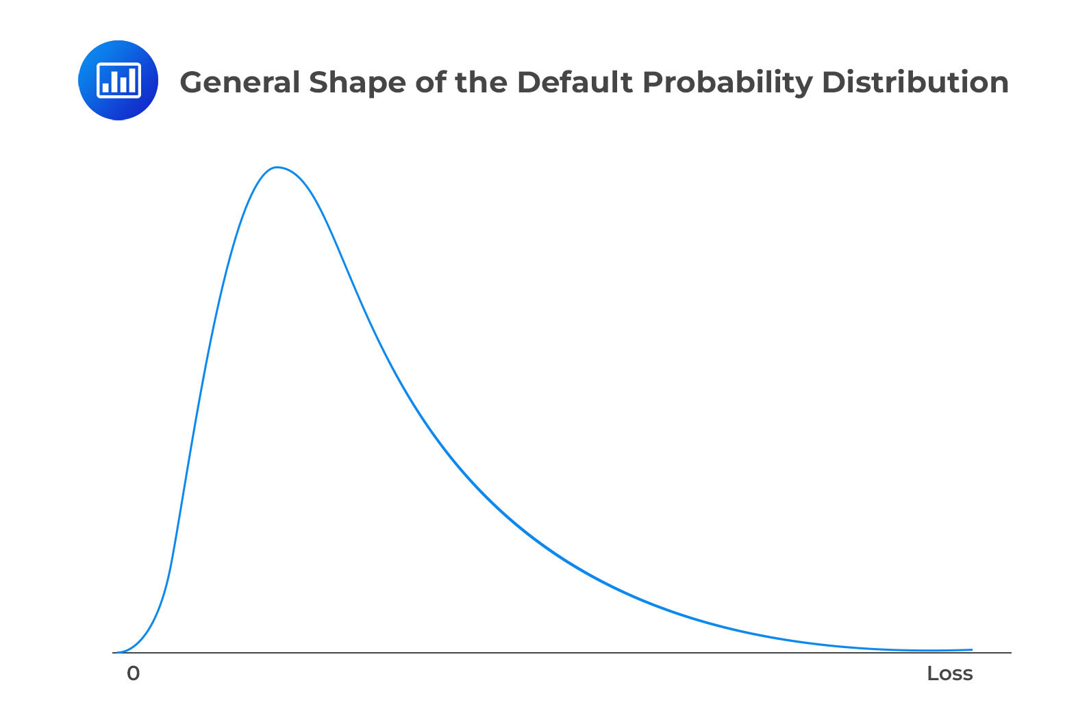
It’s crucial to emphasize that uncertainty surrounding the default rate is a critical factor in this analysis. When there’s little uncertainty, the default correlation is minimal, implying a lower likelihood of a significant number of defaults. However, as uncertainty about the default rate increases, so does the default correlation, making a substantial number of defaults more likely. This correlation arises because all companies share the same default rate, which can vary from high to low. Without default correlation, the loss probability distribution appears relatively symmetrical, but when default correlation exists, it becomes positively skewed.
 CreditMetrics
Vasicek’s model and Credit Risk Plus both estimate the probability distribution of losses stemming from defaults without considering the impact of downgrades. However, the CreditMetrics model, introduced by JPMorgan in 1997, is designed to account for both downgrades and defaults. This model relies on a rating transition matrix, which can consist of either internal ratings derived from the bank’s historical data or ratings provided by external rating agencies.
To calculate a one-year credit Value at Risk (VaR) for a portfolio of transactions involving numerous counterparties, a Monte Carlo simulation is conducted. In each simulation trial, the credit ratings of all counterparties are determined at the end of one year. Subsequently, the credit loss for each counterparty is calculated. If a counterparty’s end-of-year credit rating does not indicate default, the credit loss is determined by valuing all the transactions with that counterparty at the one-year mark. However, if the end-of-year credit rating indicates default, the credit loss is computed as the exposure at default multiplied by one minus the recovery rate.
To make these calculations, we require the term structure of credit spreads for each rating category. One straightforward assumption is that it reflects what’s currently observed in the market. Alternatively, we can assume the existence of a credit spread index with a certain probability distribution, and all credit spreads are linearly related to this index.
In cases where transactions involve derivatives, we need to extend the calculations, much like the Credit Valuation Adjustment (CVA) explained in Chapter 18. For each counterparty, we divide the time between today and the end of the longest transaction’s life into smaller intervals, with qi representing the probability of default during each interval.
In CreditMetrics, credit rating changes among different entities are considered to be correlated, not isolated events. This correlation is captured using a Gaussian copula model which helps in constructing a joint probability distribution for these changes. This ties the changes in credit ratings to the correlation observed in the companies’ equity returns, leveraging the principles of the capital asset pricing model for consistency.
For instance, when we assess the rating changes of A-rated and B-rated companies over one year, we draw two correlated variables from a standard normal distribution. These variables, let’s call them xA and xB, are set to have a correlation of 0.3, mirroring a moderate relationship between the equity returns of these companies.
The variable xA influences the new rating for an A-rated company, while xB does the same for a B-rated company. Using a probabilistic approach, we can determine the thresholds for rating changes. For example, if xA falls below a certain value, it indicates an upgrade to AAA. If it falls between two other values, it remains A-rated, and so forth.
Table 1: One-Year Ratings Transition Matrix (%)
$$\begin{array}{l|c|c|c|c|c|c|c|c}\text{Initial Rating} & \text{AAA} & \text{AA} & \text{A} & \text{BBB} & \text{BB} & \text{B} & \text{CCC/C} & \text{D} \\
\hline \text{AAA} & 88.0 & 10.0 & 1.5 & 0.3 & 0.1 & 0.05 & 0.04 & 0.00 \\
\hline \text{AA} & 0.4 & 90.0 & 8.0 & 1.0 & 0.4 & 0.15 & 0.05 & 0.01 \\
\hline \text{A} & 0.02 & 2.0 & 92.0 & 5.0 & 0.7 & 0.25 & 0.03 & 0.03 \\
\hline \text{BBB} & 0.00 & 0.2 & 4.0 & 90.0 & 4.5 & 1.0 & 0.3 & 0.01 \\
\hline \text{BB} & 0.00 & 0.1 & 0.5 & 5.0 & 85.0 & 8.0 & 1.3 & 0.1 \\
\hline \text{B} & 0.00 & 0.05 & 0.2 & 0.8 & 6.0 & 80.0 & 12.0 & 0.95 \\
\hline \text{CCC/C} & 0.00 & 0.05 & 0.03 & 0.25 & 1.3 & 15.0 & 70.0 & 12.7 \\
\hline \text{D} & 0.00 & 0.01 & 0.03 & 0.00 & 0.1 & 0.95 & 12.7 & 90.0 \end{array}$$
From the table, the probability of an A-rated company moving to AAA, AA, A, and so on is 0.02%, 2.00%, 92.00%…
In the case of an A-rated company, the highest probability remains at ‘A,’ indicating that it’s most likely that the company will maintain its current rating. The lower probabilities associated with moving to ‘AAA’ or ‘AA’ suggest that upgrades to significantly higher credit ratings are less common. Conversely, the probabilities of downgrading to lower ratings like ‘BBB,’ ‘BB,’ or ‘B’ are higher than upgrades but still less likely than remaining at an ‘A’ rating. The very low probabilities of moving to ‘CCC/C’ or defaulting (‘D’) reflect the relative rarity of such drastic downgrades over the course of a single year for a company currently rated ‘A.’
Credit spread risk is a pivotal component in the valuation of most credit-sensitive products, particularly those held in the trading book. Credit spreads, which reflect the difference in yield between credit-risky instruments and risk-free benchmarks, are critical determinants of the products’ values. When calculating Value at Risk (VaR) or Expected Shortfall (ES) for portfolios that include credit-sensitive instruments, potential credit spread changes must be taken into account.
The calculation of VaR with respect to credit spread risk could involve the historical simulation method to derive a one-day 99% VaR:
Adjusting VaR for credit spread risk is not without challenges:
Practice Question
A risk manager is comparing the calculation approaches for market risk value at risk (VaR) and credit VaR when advising a financial institution on risk assessment methods. Given that market risk VaR typically uses a one-day time horizon for trading portfolios, and historical simulation is often employed due to its simplicity in application to price movements, the manager notes the unsuitability of these methods for credit risk VaR which requires more sophisticated modeling of credit events like defaults. How should the risk manager appropriately describe the tools for measuring credit VaR compared to market risk VaR?
- Credit risk VaR uses historical simulation because it effectively models the frequency and complexity of credit events like defaults.
- Credit risk VaR employs a long time-horizon, often one year, and uses more sophisticated and elaborate models incorporating factors such as credit correlations and rating transitions.
- Market risk VaR requires a longer time horizon and more complex modeling than credit risk VaR due to the lower frequency of market price fluctuations compared to credit events.
- Both market and credit risk VaRs can utilize the same tools for measurement, as they are both based on high-frequency changes in financial markets.
Correct Answer: B
Crisk VaR usually employs a longer time horizon, often one year, reflecting the infrequency of credit events such as defaults or rating downgrades compared to daily market price fluctuations. It uses sophisticated models to address less frequent and more complex credit events, incorporating credit correlations and rating transitions to account for the interconnectedness of default risks among different companies.
A is incorrect because historical simulation, while commonly used for market risk VaR, is not suited for credit risk VaR due to the unique nature and lower frequency of credit events, which necessitates more complex modeling.
C is incorrect because it inaccurately claims that market risk VaR requires more complex modeling due to a longer time horizon when, in fact, market risk VaR typically has a shorter time horizon and credit risk VaR requires more complex modeling due to the infrequency of credit events.
D is incorrect because market and credit risk VaRs cannot utilize the same tools for measurement due to differences in the nature and frequency of market and credit events they aim to capture.
Things to Remember
- Credit risk VaR captures potential losses from credit events over a specified period, usually a year, and at a certain confidence level; it requires models that can handle credit event rarity and complexity.
- While historical simulation is popular for market risk VaR, credit risk VaR involves methods that can accommodate credit correlations and transitions due to the interconnectedness of risks among companies.
Credit Value at Risk is a core FRM Part II Credit Risk concept. Candidates may be tested on default probabilities, loss distributions, portfolio credit exposure, and how unexpected credit losses are measured under different confidence levels.
Build confidence with the FRM Part II prep course featuring guided lessons, practice questions, and realistic mock exams.
Practice FRM Part II credit risk questions covering credit VaR, portfolio loss distributions, default risk, and exam-style applications.
Offered by AnalystPrep


Get Ahead on Your Study Prep This Cyber Monday! Save 35% on all CFA® and FRM® Unlimited Packages. Use code CYBERMONDAY at checkout. Offer ends Dec 1st.