


Portfolio Construction
After completing this reading, you should be able to: Distinguish among the... Read More

After completing this reading, you should be able to:
Financial regulations have developed over the years in response to stressful periods, which exposed the weaknesses of the underlying regulations at that time. For instance, before the governments’ intervention, banks and insurance companies were created without official approval, and their success or failure depended on their strength in persuading the clients. Moreover, they tried to build a good reputation by ramming support from the prominent people in the community, accumulating a large amount of capital at their conception, and constructing prominent buildings.
Financial failures from these institutions were frequent due to insolvency and a lack of client confidence. This was clear because when the failures occurred, the clients scrambled to withdraw their funds, which, when the withdrawals caused panic, even the solvent institutions could fail if they could not liquidate their assets on time.
These failures prompted the first regulations, such as financial institutions unifying in case of excess withdrawals. Additionally, early clearinghouses were established, which were partial arrangements for mutual support. The clearing houses had the right to private inspection and hence monitoring and institutionalizing solvency.
However, the privatization of the clearinghouses’ inspection came with some drawbacks:
International trade emerged in the 1960s and 1970s, which saw the growth of the multinational corporation, and thus foreign exchange and capital flow increased. As a result, multinationals valued the financial providers in many countries, giving rise to the following problems:
Due to these problems, it was evident that the solution lay in official sector cooperation and coordination. Therefore, the Basel Committee on Banking Supervision (BCBS) was formed in 1974, just after Hertatt Bank’s failure.
Basel I accord was the specification for capital regulation developed in the late 1980s by the members of BCBS (mostly G10 nations). The accord was published in December 1987, agreed upon in July 1988, and implemented by the end of 1992. However, by early 2000, it was recognized as a global minimum capital standard.
Basel I bears no legal ground. Nevertheless, countries chose to include Basel I standards through domestic laws and regulations.
The following events triggered the Basel I accord:
The key features of Basel I are the minimum risk-based capital ratio and the numerators and denominators of this ratio.
The Basel Committee on Banking Supervision’s main goal is to ensure financial institutions have enough assets to remain solvent in times of stress. Therefore, they had to find a way of measuring this sufficiency.
The specification of the minimum capital requirement in terms of the leverage ratio (ratio of capital to book value of assets) would undermine the financial institutions with low-risk portfolios and advantage those with high-risk capital ratios. Therefore, BCBS developed a risk-based ratio. This is the ratio of capital to risk-weighted assets (RWA).
The risk-weighted assets included the assets on the balance sheet according to accounting requirements, off-balance sheet exposures (such as loan commitments), and derivative exposures.
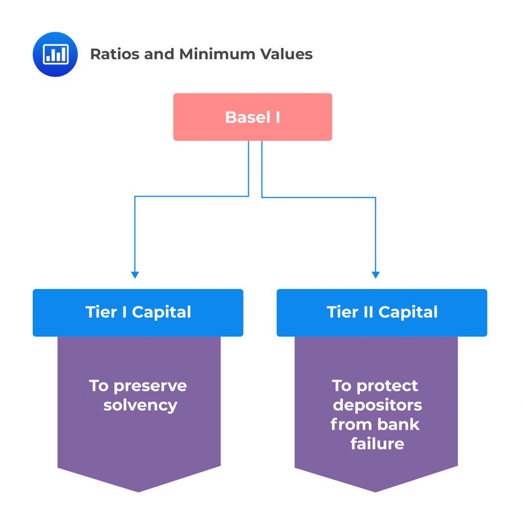
The requirement of Basel I was that the consolidated bank should maintain the following ratios:
$$ \cfrac { \text{Tier 1 capital} }{ \text{RWA} } >4\% $$
and
$$ \cfrac { \text{Total capital} }{ \text{RWA} } >8\% $$
Note that the total capital is the sum of Tier 1 and Tier 2 capital, where Tier 2 should not be more than half of the capital.
According to Basel I, Tier 1 capital is defined as common equity and disclosed reserves (retained earnings and types of the minority interest in subsidiaries) less goodwill. Some of the later Basel I frameworks include a limited amount of non-cumulative perpetual preferred stock.
The Tier 2 capital consists of the following:
The proportion of the loan reserves to be included in the capital was lowered from 2% to 1.25% of RWA.
The BCBS committee did not put forward the assumptions, but intuitively, the assumptions were:
The on-balance sheet amount of each asset was made risk-sensitive by multiplying each asset by the percentage weight according to its risk. The RWA is defined as:
$$ \text{RWA} = \sum _{ \text{i}=1 }^{ \text{N} }{ { \text{W} }_{ \text{i} }{ \text{A} }_{ \text{i} } } $$
Where:
\({\text{W}}_{\text{i}}\) = Risk weight.
\({\text{A}}_{\text{i}}\) = Size of the asset.
The weights, according to Basel I accord, are as follows:
$$\begin{array}{l|l}\textbf{Percentage Weight} & \textbf{Asset Category} \\ \hline 0\% & \text{Cash; claims on OECD governments such as bonds} \\ & \text{issued by the central government; other instrument} \\ & \text{with a full guarantee from an OECD government.} \\ \hline 20\% & \text{Claims on OECD banks and on OECD public} \\ & \text{ sector entities, such as claims on municipalities or on} \\ & \text{Fannie Mae and Freddie Mac.} \\ \hline 50\% & \text{Uninsured residential mortgage} \\ \hline 100\% & \text{All other exposures such as commercial or consumer loan}\end{array}$$
Looking at the risk weights, the maximum risk weight is 100%. Moreover, the government OECD has 0% weight implying that the government OECD would not default on its obligation.
The constituents of an Australian bank are 100 million AUD of American government bonds, 400 million AUD of loans to corporations, 300 million AUD of uninsured residential mortgages, and 250 million AUD of residential mortgages issued by the public sector. What is the value of risk-weighted assets (RWA) based on Basel I accord?
Using the weight ratios under the Basel I accord, the weights are as follows:
So that the RWA is given by:
$$ \text{RWA}=0\%\times100+100\%\times400+50\%\times300+20\%\times250=$600 \text{ million} $$
As stated earlier, RWA includes balance sheet exposures, off-balance sheet exposures, and other non-traditional on-balance sheet exposures, such as derivatives. There are two steps to determine the RW for off-balance sheet exposures:
(I) Multiply the principal amount by a credit conversion factor to get the credit equivalent (on-balance sheet equivalent) amount.
(II) Multiply the credit equivalent amount by a risk weight depending on the nature of the counterparty.
The Basel I credit conversion factors are shown below:
$$ \small{\begin{array}{l|l} \hline {\textbf{Credit} \\ \textbf{Conversion} \\ \textbf{Factor}} & \textbf{Off-Balance sheet Asset Category} \\ \hline {100\%} & {\text{Guarantees on loans and bonds, bankers acceptances and equivalents}} \\ \hline {50\%} & {\text{Warrantees and standby letters of credit related to transactions}} \\ \hline {20\%} & {\text{Loan commitments with an original maturity greater than or equal to one year}}\\ \hline {0\%} & {\text{Loan commitments with original maturity less than one year} } \\ \end{array}}$$
For example, OECD municipalities are subject to a risk weight of 20%. Therefore, a $200 million five-year loan commitment to an OECD municipality implies that the credit equivalent amount is $40 million (i.e., 20% × $200 million). The loan’s contribution to RWA is thus $8 million (i.e., 20% × $40 million).
In the case of derivative instruments, the Basel I offered two methods of calculating credit equivalent amount:
Note that the credit equivalent amount was amended in 1995 to include maturities of over five years.
The steps of calculating the credit equivalent of the derivative under this method include:
The original exposure method was specifically for interest rate and foreign exchange contracts. The steps included:
It is worth noting that equity and commodity derivatives were not included in Basel I and that the risk weight was determined based on the counterparty while making sure that no weight exceeded 50%.
The derivatives book of an American bank consists of three interest rate swaps, each with a notional value of $200m and maturities of 0.5, 1.5, and 2.5 years, respectively. The market value of swaps is $30 million. Additionally, the book contains $300 million of foreign exchange swaps, with each $100 million having the same maturity description as in interest swaps.
Calculate the credit equivalent amount of the bank’s derivatives book.
Using the description given:
$$ \text{V} = 30 $$
For the value of the swaps:
$$ \text{D} = 0\% \times 200 +0.5\% \times 400=$2 \text{ million} $$
For the foreign exchange swaps:
$$ \text{D} = 1\% \times 200 +5\% \times 400=$11 \text{ million} $$
Thus, the Credit equivalent is given by:
$$ \text{CE}=30+2+11=$43 \text{ million} $$
The handling of the derivative exposures by Basel I was basic. However, by 1995 much had changed after the 1987 stock crash, the rising popularity of the VaR, and the existence of developed quantitative market risk management systems. The Market Risk Amendment revolved around the issues of netting and capital for market risks associated with trading activities.
In a conventional market, the entities that transact in over-the-counter derivatives sign an International Swaps and Derivatives Association. The agreement states that in case one party defaults in its obligations, the transaction of the defaulting party with its counterparty is considered a single transaction. Moreover, depending on the choices in the transactions, the agreement allows bilateral transactions with negative and positive values to offset one another. For instance, if two entities, A and B, enter an interest swap agreement against interest movements, the overall net exposure in each of the entities is zero if the interest rate does not move. Thus the value of the portfolio is zero.
The initial Basel I did not incorporate the capital credit for netting. Conventionally, the changes in interest would have an offsetting effect on the market value of two swaps. Still, Basel I would include an add-on in each swap, discouraging the hedging strategy. The reason behind this strategy was that bankruptcy courts had not sufficiently tested the master agreements.
By 1995, the BCBS members were confident that “add-on” agreements would work as required. Thus, the 1995 amendment incorporated reductions in the credit equivalent amounts when enforceable bilateral netting agreements were set.
When calculating the equivalent amount, complete netting of the market values of all positions was allowed for each counterparty i, and add-on Dj for the future changes in the value was decreased for each category of derivative j. So, the credit equivalent amount (CEA) is given by:
$$ \text{CEA} = {\text{max}\left( \sum _{ \text{i}=1 }^{ \text{N} }{ { \text{V} }_{ \text{i} },0 } \right) } + \sum _{ \text{j} }^{}{ {\left(0.4\times {\text{D}}_{\text{j}} + 0.6 \times {\text{D}}_{\text{j}} \times \text{NRR}\right) } }$$
Where NRR (Net Replacement Ratio) is defined as:
$$ \text{NRR} =\cfrac { \text{max}\left( \sum _{ \text{i}=1 }^{ \text{N} }{ { \text{V} }_{ \text{i} },0 } \right) }{ \sum _{ \text{i}=1 }^{ \text{N} }{ \text{max}\left( { \text{V} }_{ \text{i} },0 \right) } } $$
Note that \({ \text{max}\left( \sum _{ \text{i}=1 }^{ \text{N} }{ { \text{V} }_{ \text{i} },0 } \right) }\) (numerator) is the market value of positions of type j with netting while \(\sum _{ \text{i}=1 }^{ \text{N} }{ \text{max}\left( { \text{V} }_{ \text{i} },0 \right) } \) (denominator)is the market value with no netting.
NRR is the average across the positions. The add-on and effect of netting differences across different derivatives were ignored.
Assume that a bank has a portfolio of four derivatives with two counterparties, as shown in the table below:
$$\small{ \begin{array}{l|c|c|c|c|c} \textbf{Counterparty} & {\textbf{Derivative}\\ \textbf{type}} & \bf{\text{Maturity} \\ \text{Period}} & \bf{\text{Notional} \\ \text{Amount}} & \bf{\text{Market } \\ \text{Value}} & {}\\ \hline {1} & \text{Interest rate} & {2} & {100} & {-5} & {0.10\%} \\ \hline {1} & \text{Interest rate} & {2} & {200} & {14} & {0.10\%} \\ \hline {2} & \text{Equity Option} & {3} & {100} & {0} & {10\%} \\ \hline {2} & \text{Wheat Option} & {6} & {200} & {-10} & {5\%} \\ \end{array}}$$
What is the value of the credit equivalent of the derivative portfolio?
We know the credit equivalent is given by:
$$ \text{CEA} = {\text{max}\left( \sum _{ \text{i}=1 }^{ \text{N} }{ { \text{V} }_{ \text{i} },0 } \right) } + \sum _{ \text{j} }^{}{ {\left(0.4\times {\text{D}}_{\text{j}} + 0.6 \times {\text{D}}_{\text{j}} \times \text{NRR}\right) } }$$
Now,
$$ {\text{max}\left( \sum _{ \text{i}=1 }^{ \text{N} }{ { \text{V} }_{ \text{i} },0 } \right) } = \text{max} \left(0,9\right) =9 $$
Note that the current exposure portion of the credit equivalent is 9 for counterparty 1 because -5 exposure on the first interest rate is netted against 14 on the second interest rate. Moreover, the current exposure for counterparty 2 is 0 current since exposure cannot be negative (-10).
Now,
$$ \text{NRR}=\cfrac {\text{max}\left( \sum _{ \text{i}=1 }^{ \text{N} }{ { \text{V} }_{ \text{i} },0 } \right) }{ \sum _{ \text{i}=1 }^{ \text{N} }{ \text{max}\left( { \text{V} }_{ \text{i} },0 \right) } } =\cfrac { \text{Current exposure} }{ \text{Sum of positive Exposure} } =\cfrac { 9 }{ 14 } =0.6429 $$
The add-on for the potential future exposures is calculated for each derivative:
$$ \begin{align*} \text{Interest rate} & =0.10\% \left(100+200 \right)=0.3 \\ \text{Equity Option} & =10\%\times100=10 \\ \text{Wheat Option} & =5\%\times200=10 \end{align*} $$
So,
$$ \begin{align*} & =\sum _{ j }^{ }{ \left( 0.4\times { \text{D} }_{ \text{j} }+0.6\times { \text{D} }_{ \text{j} }\times \text{NRR} \right) } \\ &=\left[0.4\times0.3+0.6\times0.3\times0.6429\right]+\left[0.4\times10+0.6×10\times0.6429\right] \\ & +\left[0.4\times10+0.6×10\times0.6429\right] \\ & =0.2357+7.8574+7.8574=15.95 \end{align*} $$
Therefore,
$$ \text{CEA}=\text{max}\left( \sum _{ \text{i}=1 }^{ \text{N} }{ { \text{V} }_{ \text{i} },0 } \right) +\sum _{ j }^{ }{ \left( 0.4\times { \text{D} }_{ \text{j} }+0.6\times { \text{D} }_{ \text{j} }\times \text{NRR} \right) } =9+15.95=24.95 $$
In the initial description of Basel I, market risk is left out. Recall that market risk is a potential change in the market value of trading book values.
The Amendment of Basel I gives two ways to measure market risk:
The internal model’s approach is suitable for banks with material-size trading books because it generated lesser capital requirements since the asset values were assumed to be uncorrelated as they were in a standardized approach.
The standardized approach explains the following classification of positions separately:
Note that the internal models-based method allows the banks to use their own internally developed risk measures as the inputs. On the other hand, the standardized approach explained is based on observable features of positions, such as remaining maturity.
Under both approaches, capital charges were computed distinctively for specific risk (SR) and general market risk (MR) for each of the five categories stated above. The SR and the MR were then summed and then multiplied by 12.5 so that the usual multipliers on RWA could be applied to them. It is worth noting that 12.5 is the inverse of 8% so that the multiplier transforms the capital requirements into an RWA measure with particular attention to total capital. So the capital charge is given by:
$$ \text{Total capital for trading assets}=0.08\times 12.5\sum _{ \text{j}=1 }^{ 5 }{ \left( { \text{MR} }_{ \text{j} }+{ \text{SR} }_{ \text{j} } \right) } $$
For a bank using an internal model-based approach, the bank is obliged to calculate the value at risk (VaR) for each asset category. According to the amendment, a 10-day 99% VaR was required on one year of daily data, usually using a scale of √10.
Therefore, the market risk is given by:
$$ \text{MR}=\text{max}\left( { \text{VaR} }_{ \text{t}-1 },\text{m}\times { \text{VaR} }_{ \text{avg} } \right) $$
Where:
\({\text{VaR}}_{\text{avg}}\) = average VaR over the past 60 days.
m = multiplier that was not less than 3 (but can be more than 3).
Capital for specific risks required for fixed income could be computed using a standardized approach or the bank’s internal models. However, if the internal models were used, the method would be similar to that of market risk, but the multiplier would be 4 rather than 3.
The 1996 amendment introduced Tier 3 capital, which consisted of unsecured subordinated debt with an initial maturity of at least two years that could be utilized to cover the market risk requirements. However, only 70% of the market risk capital requirements could be covered by Tier 3 capital.
The 1996 Amendment concentrated on the requirements of the banks using the internal model-based approach. For instance, the amendment required the banks to have sound risk management and independent risk management units.
Moreover, the 1996 amendment required daily backtesting. For each model, the banks were required to compute one-day 99% VaR for each of the significant 250 days and draw a comparison between the actual loss for the day and the VaR. If, for a day, the actual loss is larger than VaR, it is termed as an exception. For less than five exceptions, the multiplier was taken to be 3. However, for more than five exceptions, the supervisor has the option to choose larger multipliers, but for ten or more exceptions, a multiplier of 4 was recommended.
By the mid-1990s, some supervisors had become alarmed that Basel I was not risk-based enough as it claimed to be. For instance, the 100% risk weight included exposures that put the corporations at a variety of risks.
Moreover, the banking crisis in Nordic countries proved that the issues could occur in banks with sound chaptalization. Additionally, there was an advancement in market and credit risk quantification and management from 1987 onwards, which incentivized accurate risk weighting and risk management at all hierarchies of banking institutions.
As a result, Basel II was initiated in the late 1990s, and the finalized version was published in 2004 and later revised several.
The Basel II Accord contained the following significant improvements:
The Basel II pillars formed a basis for common national practices. Pillar 2 mandated the supervisors to ensure that banks possess more than the minimum amount of capital and the internal capital adequacy process (ICAAP) that considers their risk profile. The supervisors were required to act on the earlier signs that the bank’s capital would go below the minimum by recommending appropriate actions. Moreover, the supervisors were required to motivate the banks to improve the risk management systems and adequately address the deficiencies.
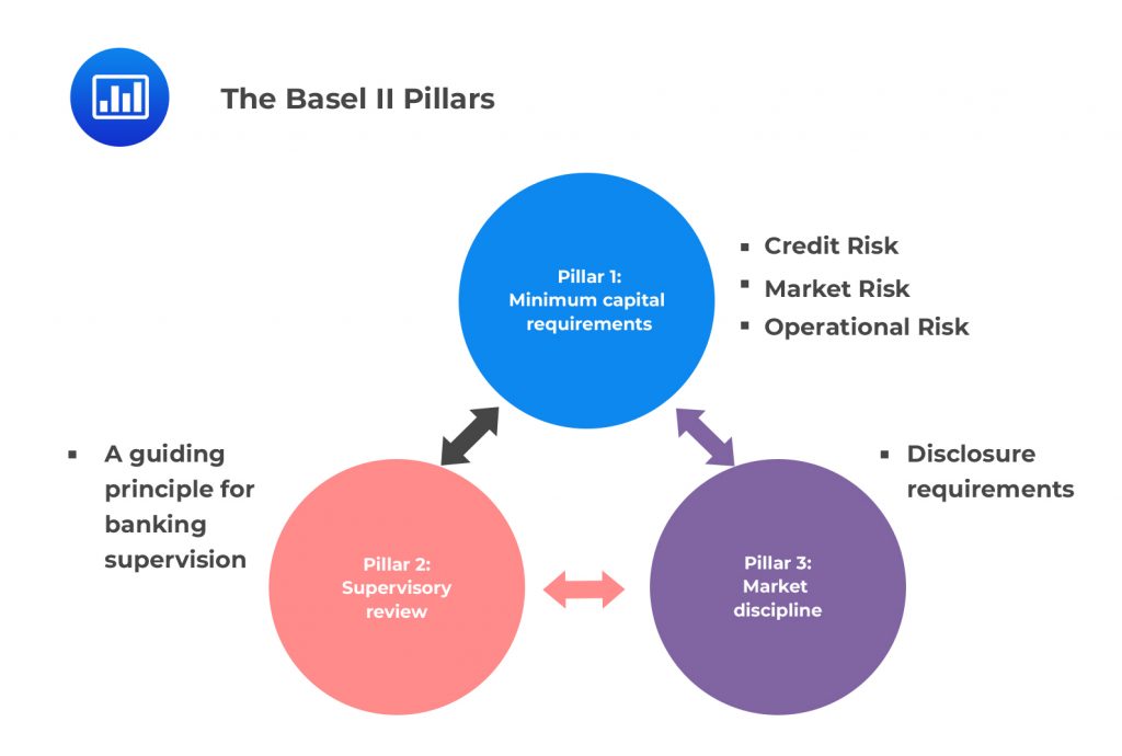 Pillar 3 advocated for more qualitative and quantitative disclosures with the aim that the market participants’ pressures would assist in improving the bank’s practices. It required qualitative disclosures such as corporate structure, the applicability of the Basel accord, and accounting procedures. The quantitative disclosures include the features of the bank’s capital, risk measures, and exposures.
Some banks found the pillars challenging to interpret, and the disclosure practices were not uniform over the years, but Basel emphasized them while providing more clarity.
Supervisors were wary that the banks could distort the interval risk measure to lower the required capital due to a lack of sufficient supporting data and analysis in Basel II. Therefore, the negotiators introduce three methods of determining minimum capital requirements to cover credit risk:
This method was directed to banks with internal risk measures and risk management systems that were insufficient to support IRB methods. The risk weights were sensitive to fluctuation in risks. Unlike the Basel I standardized approach, whose risk weights were based on asset type and the country to which the obligor belongs, Basel II risk weights depended on the type of the obligor, ratings of some obligors, and asset types of some obligors. The table below shows some examples of some risk weights
$$ \begin{array}{l|c|c|c|c|c|c} \textbf{Obligation of:} & {\textbf{AAA to}\\ \textbf{AA-}} & \textbf{A+ to A-} & \bf{\text{BBB+ to} \\ \text{BBB-}} & \bf{\text{BB+ to} \\ \text{BB-}} & \textbf{B+ to B-} & \textbf{Unrated}\\ \hline \text{Countries} & {0} & {20} & {50} & {100} & {150} & {100} \\ \hline \text{Banks} & {20} & {50} & {50} & {100} & {150} & {50} \\ \hline \text{Corporations} & {20} & {50} & {100} & {100} & {150} & {100} \\ \end{array} $$
As seen above, the weights were somewhat severe for the banks as compared to Basel I, but the severity could be lowered at the national discretion. For instance:
The Basel II standardized included two methods for adjusting for collateral:
The simple approach is similar to Basel I in that the risk weight of a counterparty could be substituted with the risk weight of collateral for the proportion of the exposure covered by the collateral. The minimum collateral weight was 20%, except for the collateral, which sovereign debt collateral expressed in the same currency as the exposure.
The comprehensive approach required variations of the exposures and the collateral amounts to incorporate the possible value deviations. That is, the risk weight of the collateral was applied to the minimum collateral, and the counterparty’s risk weight was applied to the remaining exposure. Moreover, netting was applied distinctively to exposures and collaterals, and either Basel or approved internal models could be applied to facilitate the adjustments.
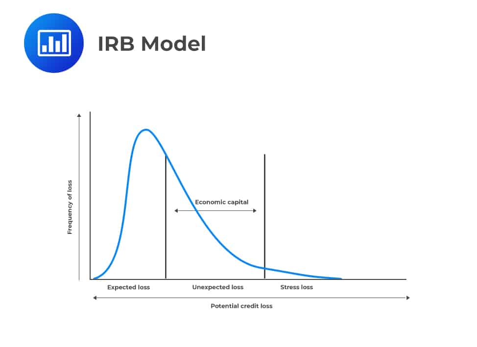
The IRB model is based on Gordy’s (2003) one-factor Gaussian copula model. Gordy postulated that, given a well-diversified portfolio, there exists a positive link between the default probability of an obligor and the obligor’s contribution to the capital required to cap the probability of the portfolio losses surpassing the loss distribution percentile.
The Basel committee chose a one-year time horizon for the credit losses and desired \({99.9}^{\text{th}}\) percentile credit loss distribution. So the formula for the capital required for credit risk is given by:
$$ \text{Capital}=\sum \left[\text{EAD}_\text{i}\times \text{LGD}_\text{i} \times \text{DR}{99.9}_{\text{i}} \right]-\text{EL} $$
Where
\({\text{EAD}}_{\text{i}}\) = the exposure at default for an asset i, that is, the amount expected to be owed by the counterparty on an asset i in case of a default
\({\text{LGD}}_{\text{i}}\) = expected loss given default for asset i (expected proportion of \({\text{EAD}}_{\text{i}}\) to be lost)
\(\text{DR}{99.9}_{\text{i}}\) = default rate at the \({99.9}^{th}\) percentile for a large portfolio of assets of category i. This quantity is defined as:
$$ DR_{99.9} = N\left( \frac{N^{-1}(\text{PD}) + \sqrt{\rho} \cdot N^{-1}(0.999)}{\sqrt{1-\rho}} \right) $$
EL= expected loss (annual credit loss) on a portfolio and defined as:
$$ \text{EL}=\sum \left[\text{EAD}_\text{i}\times \text{LGD}_\text{i} \times \text{PD}_{\text{i}} \right] $$
Note that the capital was expressed in terms of dollars.
The Basel Committee did not consider the loan reserves as part of Tier 1 capital, but the loan reserves were taken to be approximately equivalent to the expected loss.
Therefore, the committee decided to make the capital the function of the unexpected losses (net expected losses). When loan reserves were less than expected losses (EL), the capital was reduced for the shortfall.
 Consequently, the Basel Committee was able to state the loss percentile and the asset correlation (\(\rho\)) for each asset category. Therefore, the contribution of each asset to the capital was based only on the bank’s estimates of EAD, LGD, and PD for a particular asset.
There were two types of IRB models:
Bank, Corporate, and Sovereign Exposure Under IRB
Basel II assumes that the correlation (ρ) and the probability of default (PD) depend on Lopez’s (2004) model, which defines the correlation as:
$$ \rho =0.12\left[ \cfrac { 1-{ \text{e} }^{ -50\text{PD} } }{ 1-{ \text{e} }^{ -50 } } \right] +0.24\left[ 1-\cfrac { 1-{ \text{e} }^{ -50\text{PD} } }{ 1-{ \text{e} }^{ -50 } } \right] $$
Lopez’s model gives the relationship between the average asset correlation, the firm’s PD, and the asset size. Looking at the formula above, the average asset correlation decreases as PD increases, confirming that the default for high-risk borrowers is usually idiosyncratic. In contrast, middle-class borrowers tend to default when the aggregate economy is in distress. Moreover, the safest borrowers are also idiosyncratic, but their default rates (DR) are ignored since they are usually minimal.
The computation of capital for banks, corporate, and sovereign exposures incorporates the maturity adjustment to account for the assets with maturity more than one year of remaining maturity, which usually remains on the balance sheet at the end of the loss-forecasting period and may have lowered in credit quality. The Maturity adjustment is given by:
$$ \text{MA}=1+\cfrac { \text{b}\left( \text{M}-2.5 \right) }{ 1-1.5\text{b} } $$
Where:
MA = Maturity of the asset.
\(\text{b}=\left[0.11852-0.05478 \text{ln(PD)} \right]^{2}\)
Now, recall that the Basel II expressed the required capital in terms of RWA; the RWA for the banks, corporations, and sovereign exposures is given by:
$$ \text{RWA}=12.5\times \text{EAD} \times \text{LGD}\times \text{(DR-PD)} \times \text{MA} $$
An American bank’s assistance consists of $200 million BB-rated drawn loans. The MA is estimated to be 1.25. The probability of default is estimated to be 0.02, the LGD is 40%, and DR is estimated to be 0.15.
What is the RWA for the bank with regard to the Basel II accord?
We know that:
$$ \begin{align*} \text{RWA} & =12.5\times \text{EAD} \times \text{LGD}\times \text{(DR-PD)} \times \text{MA} \\ & =12.5\times 200\times 0.4\times \left(0.15-0.02\right)\times 1.25 \\ & =$162.5 \text{ million} \end{align*} $$
The retail exposures were calculated similarly to that of advanced IRB, only that there is no maturity adjustment. Moreover, a set of three correlations are used: ρ=0.15 for the residential mortgages, ρ=0.04 for qualifying assets (such as credit card balances), and other retail assets. The correlation is defined as:
$$ \rho =0.03\left[ \cfrac { 1-{ \text{e} }^{ -35\text{PD} } }{ 1-{ \text{e} }^{ -35 } } \right] +0.16\left[ 1-\cfrac { 1-{ \text{e} }^{ -35\text{PD} } }{ 1-{ \text{e} }^{ -35 } } \right] $$
Looking at the formula, it is evident that the correlations are lower for retail than wholesale exposures.
An American bank’s assets consist of $200 million BB-rated drawn loans. The probability of default is estimated (PD) to be 0.02, the LGD is 40%, and DR is estimated to be 0.10.
What is the RWA for the bank with regard to the Basel II accord?
Recall that retail exposures were calculated similarly to that of advanced IRB, only that there is no maturity adjustment. So,
$$ \begin{align*} \text{RWA} & =12.5\times \text{EAD} \times \text{LGD}\times \text{(DR-PD)} \\ & =12.5\times 200\times 0.40\times \left(0.10-0.02\right)=$80 \text{ million} \end{align*} $$
A credit substitution was utilized for arrangements such as guarantees and credit default swaps. This method involved substituting the credit rating of the guarantor for that of the obligor in the capital calculations until the amount covered by the mitigant is reached.
However, this method has low sensitivity to actual loss occurrence because it involves double default (guarantor and the borrower). Nevertheless, Basel II assumes low correlations of the wholesale counterparty defaults, and thus the frequency of double defaults is low.
Alternatively, the Basel Committee amendment in 2005 allowed capital without the mitigant to be multiplied by 0.15+160\({\text{PD}}_{\text{g}}\) where \({\text{PD}}_{\text{g}}\) is defined as the one-year PD of the guarantor.
According to the Basel Committee, “operational risk is the risk that occurs due to inadequate or failed internal processes, people and systems or from external events.”
Basel II implemented three methods of determining the capital required for the operational risk:
The sample of four business lines, their corresponding multipliers, and gross income (in millions) is given in the table below:
$$ \begin{array}{l|c|ccc} \textbf{Business Line} & \textbf{Multiplier}& \textbf{Annual} & \textbf{Gross} & \textbf{Income} \\ {} & {} & \text{Year 1} & \text{Year 2} & \text{Year 3} \\ \hline {\text{Retail Banking}} & {13\%} & {10} & {20} & {10} \\ \hline {\text{Asset Management}} & {14\%} & {10} & {10} & {20} \\ \hline {\text{Trading and Sales}} & {19\%} & {10} & {-50} & {30} \\ \hline {\text{Corporate Finance}} & {18\%} & {50} & {30} & {60} \\ \end{array} $$
What is the value of the required capital for operational risk under the Basic Indicator Approaches and the Standardized Approach?
Under the Basic Indicator Approach, the bank computes the capital for operational risk as 15% of the bank’s average annual gross income over the past three years while ignoring years that resulted in negative gross income.
So,
$$ \small{\begin{array}{c|ccc} \hline \textbf{Business Line} & \textbf{Annual} & \textbf{Gross} & \textbf{Income} \\ {} & {\text{Year 1}} & \text{Year 2} & \text{Year 3} \\ \hline {\text{Retail Banking}} & {10} & {20} & {10} \\ \hline {\text{Asset Management}} & {10} & {10} & {20} \\ \hline {\text{Trading and Sales}} & {10} & {-50} & {30} \\ \hline {\text{Corporate Finance}} & {50} & {30} & {60} \\ \hline {\textbf{Sum}} & \textbf{80} & \textbf{10} & \textbf{120} \\ \end{array}}$$
Note that the multiplier column has been excluded since we do not need it here. Therefore, the required capital for the operational risk is given by:
$$ 0.15\left[ \cfrac { 80+10+120 }{ 3 } \right] =10.5 \text{ million} $$
Under the Standardized Approach, it is similar to the basic indicator method, but the multipliers are distinct for each business line. So,
$$\small{\begin{array}{l|c|ccc|ccc} \textbf{Business} & \textbf{Multiplier}& \textbf{Annual} & \textbf{Gross} & \textbf{Income} & {} & {\textbf{Capital}} & {} \\ \textbf{Line} & {} & \text{Year 1} & \text{Year 2} & \text{Year 3} & \text{Year 1} & \text{Year 2} & \text{Year 3} \\ \hline {\text{Retail} \\ \text{Banking}} & {13\%} & {10} & {20} & {10} & {1.3} & {2.6} & {1.3} \\ \hline {\text{Asset} \\ \text{Management}} & {14\%} & {10} & {10} & {20} & {1.4} & {1.4} & {2.8} \\ \hline {\text{Trading and} \\ \text{Sales}} & {19\%} & {10} & {-50} & {30} & {1.9} & {-9.5} & {5.7} \\ \hline {\text{Corporate} \\ \text{Finance}} & {18\%} & {50} & {30} & {60} & {9.0} & {5.4} & {10.8} \\ \hline {\textbf{Sum}} & {} & {} & {}& {} & \textbf{13.6} & \textbf{-0.1} & \textbf{20.60} \\ \end{array}}$$
Note that the negative capital offsets the positive capital within a given year and is thus ignored. So the required capital under the standardized approach is given by:
$$ \cfrac { 1 }{ 2 } \left[ 13.6+20.6 \right] =\text{17.10 million} $$
The banks that choose to use the AMA approach are required to approximate the distribution of the operational risk losses in seven classes that include both the estimates of occurrences and severity of the loss events. The classes of operational losses are:
Although banks use different AMA approaches, the most used methods are:
Scenario analyses are merited to create an informative scenario, and they look into the future (forward-looking). However, the data used is small, and thus generating the 99.9th percentile loss is a challenging task.
Minimum capital requirements for insurance companies are present in many countries. However, there are no international standards, but the United States and the European Union have implemented some complex standards.
The US-based National Association of Insurance Commissioners (NAIC) enacted capital requirements that predicted some features of Basel II. Moreover, capital requirements on the risky assets depended on the ratings given by NAIC on each asset, which was additional to capital requirements on the liabilities. The insurance level was at the state level, where most of the states have implemented these requirements.
The European Insurance and Occupational Pensions Authority (EIOPA) regulates insurance companies in the European Union. The first capital requirement at the EU level was termed Solvency I, which Solvency II later replaced.
Solvency II is similar to Basel II in many aspects. For instance, the capital requirements are based on the one year, 99.5% VaR, and have three pillars:
Moreover, when underwriting the risks, market, credit, and operational risks are taken into consideration, which is further segmented into risks originating from life, property, casualty, and health insurance.
Solvency II also borrows some Basel II elements. For instance, it requires controls on capital. In case an insurance company breaks the Solvency II minimum capital requirement (MCR), the supervisors are advised to stop the stressed firm from accepting new policies or putting them into resolution. When a firm is put in resolution, it can either be liquidated or sold to a stronger firm.
The required buffer above the minimum capital requirement (MCR) is provided by the Solvency Capital Requirement (SCR), which is less than MCR. In case the SCR requirement is breached, the concerned insurance company should give a detailed recapitalization plan, and the supervisor might impose more requirements.
It is worth noting that Solvency II uses both standardized and internal model-based approaches to compute SCR. However, the models used must take into consideration the following factors:
Solvency II can be made to fruition through a combination of Tier 1, Tier 2, and Tier 3 capital.
Practice Question
Maria Thompson is a risk analyst at Eastview Commercial Bank. The bank’s portfolio includes $750 million in corporate loans, primarily to large businesses in various industries. The bank’s risk management team has estimated that the probability of default (PD) is 11.1% and the loss given default (LGD) is 45%. The correlation parameter is 0.135.
Based on the Basel II accord, what is the default rate at the 99.9th percentile for the bank?
A) 23.82%
B) 53.90%
C) 24.50%
D) 46.10%
The correct answer is: D)
The default rate at the 99.9th percentile (\(DR_{99.9}\)) for Eastview Commercial Bank is calculated using the formula:
$$ DR_{99.9} = N\left( \frac{N^{-1}(\text{PD}) + \sqrt{\rho} \cdot N^{-1}(0.999)}{\sqrt{1-\rho}} \right) $$
Given:
- Probability of default (\(\text{PD}\)): 11.1% or 0.111
- Correlation parameter (\(\rho\)): 0.135
Using a standard normal distribution table or a calculator, we find:
- \(N^{-1}(0.111) \approx -1.2265\)
- \(N^{-1}(0.999) \approx 3.0902\)
Plugging these values into the formula, we get:
$$\begin{align} DR_{99.9} &= N\left( \frac{-1.2265 + \sqrt{0.135} \cdot 3.0902}{\sqrt{1-0.135}} \right) \\ &= N\left( \frac{-1.2265 + 0.3674 \cdot 3.0902}{0.9302} \right) \\ &= N\left( -0.09794\right) \end{align}$$
Using the standard normal cumulative distribution function, we find:
$$ DR_{99.9} \approx N(-0.09794) \approx 0.4610$$
Therefore, the default rate at the 99.9th percentile for Eastview Commercial Bank is approximately 46.10%.
Offered by AnalystPrep


