


The Cyber-Resilient Organization
After completing this reading, you should be able to: Describe elements of an... Read More

After completing this reading, you should be able to:
Model risk is the likelihood of making incorrect investment or risk management decisions due to model errors and how the models are used. A good example of model risk is the application of a VaR implementation that depends on the assumption that returns are normally distributed without recognizing a model’s deviation from reality. Apart from the assumption that returns are normally distributed, other limitations of VaR include:
Apart from VaR, this chapter deals with the whole problem of model risk. That is the fact that models can produce errors or can sometimes be used inappropriately.
In the process of trading and investing, models are not only applicable to risk measurement alone, but also to other parts of the process. Model risks can lead to trading losses, as well as legal, reputational, accounting, and regulatory issues.
There are various ways through which errors can be introduced to models. For instance, a model’s algorithm might contain errors due to bugs in its programming. An example of model risk due to programming errors is Moody’s Rating Agency. In this case, due to their rating model, Moody’s Rating Agency awarded triple-A rating to specific structures credit products using flawed programming. As a result, Moody faced not only reputational risk but also liquidity risk. This was because once the errors became public, there was a feeling that Moody tailored the ratings to desired ratings and consequently bloated their reputation.
There is yet another example. Once, AXA Rosenburg Group LLC, which was the branch of asset management of French insurance company AXA, discovered a programming error in the quantitative investment approach. The error had caused losses to some investors. This error was not communicated to the investors on time, resulting in the loss of assets under their management. As a result of this, their reputation was tarnished.
Note that a model can be correctly coded but used inconsistently with its intended purpose. For instance, mapping positions of the risk factors might lead to differences in VaR results.
Model errors can manifest in the valuation of securities or in hedging, which leads to hidden losses within a firm or from external stakeholders. Valuation errors due to the usage of faulty models are examples of market risk and operational risk.
Valuation errors, as market risk, occur when, for example, they suggest the purchase of securities that seemingly have low prices but are fairly priced or overpriced in the real sense. On the other hand, valuation errors can pose an operational risk by making it difficult to value some securities accurately. As a result, some positions might be recorded as profitable, when, in fact, they are non-profitable.
Model errors can be evaded, and valuation risk reduced, by using the actual market prices rather than model prices. However, this is unsuitable because this approach means we are marking to market and never marking to model. For instance, long-term bank commercial loans can be difficult to mark to market because they rarely trade.
A wide range of practical drawbacks affects VaR. Computer systems are crucial in the management of risk since they automate data combination and calculation processes, and generate reports. However, data preparation is a problem associated with the implementation of risk-measurement systems, and the following three types of data are involved:
Data should be correctly matched and presented to a calculation engine using software in order to calculate a risk measure. All the applied formulas or calculation procedures will be incorporated into the computation engine, and the results conveyed to a reporting layer to be read by managers. The variability of the resulting measures and the challenge of the appropriate application of data are the issues to be focused on.
A risk manager has to be flexible to adapt their VaR computation model to suit a company’s needs, investor’s needs, or the nature of the portfolio. However, the following challenges may arise:
When these parameters are varied, changes obtained in VaR can be dramatic. VaR estimates published by some large banks are generally accompanied by backtesting results and are generated for the purposes of regulation.
VaR results can be affected by the mapping of the assignment of risk factors to positions. Some mapping decisions are pragmatic choices among alternatives, with each having its pros and cons.
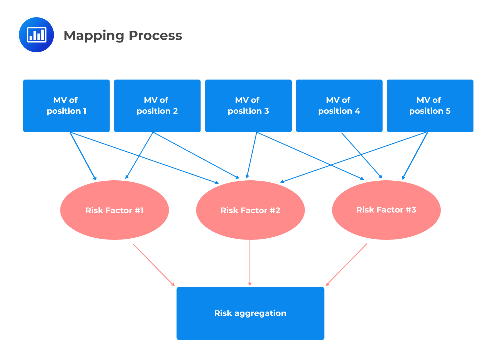
Difficulties in the handling of data that address some risk factors may be experienced in some cases. Such challenges merely reflect the actual difficulties of hedging or expressing some trade ideas. Convertible bond trading can, for example, be mapped to a set of risk factors such as implied volatilities and credit spreads. The basis of such mappings is the theoretical price of convertible bonds. Sometimes, however, there can be a dramatic divergence of the theoretical and market prices of converts. The divergences are liquidity risk events that are not easily captured by market data. This implies that risk can be drastically understated since the VaR is based solely on the replicating portfolio.
The same risk factors or set of risk factors can, in some instances, be mapped into position and its hedge. This is in spite of the justification that the available data makes it difficult to differentiate two closely related positions. Despite there being a significant basis risk, the result will be a measured VaR of zero. An excellent example of basis risk is risk modeling of securitization exposure, which is usually related hedged corporate CDS indexes. That is, if the underlying exposures are mapped to a corporate spread time series, then the measured risk vanishes.
For some strategies, VaR can be misleading due to the distribution of returns and VaR’s dependence on specific modeling choices. Nevertheless, for other strategies, outcomes are close to binary. Event-driven strategies (those that depend on events such as lawsuits) and dynamic strategies (strategies where the trading strategy creates the risk as time goes by rather than the positions) are examples of strategies whose outcomes are close to binary.
The 2005 credit markets’ volatility episode is a perfect case study of model risk stemming from the misinterpretation and misapplication of models. According to the model, one dimension of risk was hedged, yet other risk dimensions were neglected. This caused large losses to various traders.
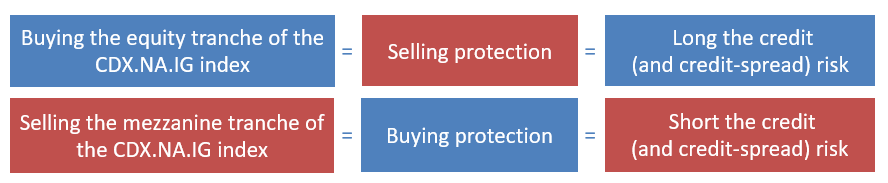
The selling of protection on the equity tranche (riskier) and the purchasing of protection on the junior mezzanine tranche (less risky) of the CDX.NA.IG was a widespread trade among various market players. The trade was, therefore, long credit and credit-spread risk through the equity tranche and short credit and credit-spread risk through the mezzanine. The design of the model was that at initiation, it should be default-risk-neutral, by sizing the two legs of the trade for their credit spread sensitivities equally.
 Profiting from a view on credit spread was not the trade’s motivation, despite it being market-risk oriented. It was instead designed to achieve a positively convex payoff profile. The volatility of the credit spread would then benefit the portfolio of the two positions.
Using the previously developed tools, we can better understand the trade and its risks by setting up trade-in tranches of the illustrative Collateralized Loan Obligation (CLO) which is structure-wise, and motivation-wise, similar to the previously described standard tranche. Note that we would unlikely take a short position in cash securitization since the bond will be hard to locate and borrow. Therefore, we resort to buying protection through credit default swap (CDS). Also of notable interest is the fact that the dealer of the CDS might charge more to compensate for the illiquidity of the product, the difficulty of hedging it, and correlation risk. The standard tranches are synthetic CDS with their collateral pools consisting of CDS. Being more liquid than most other structured products enables traders to take both long and short positions in these products.
Assuming that we now want to determine the amount of mezzanine we are supposed to short (hedge ratio), we utilize the default sensitivities, defualt01s. The 2005 CDX trade utilized market-risk sensitivity termed as the spreads01s. However, the methodologies of hedging are similar.
Now, assume that at the start of the trade, the default risk \(\pi\)=0.04, and the implied correlation \(\rho\)=0.40. Then the default01 of a $100,000 notional position in the equity trench is -$6,500, and that of the mezzanine is -$800 so that the hedge ratio is \(\frac{-6500}{-800}=8.125\). That is, if we short 8.125×100,000=812,500 of the par value of the mezzanine for a given $100,000 notional value of a long, then we would have created a portfolio that is default risk-neutral.
In an actual standard tranche trade, the methodology is a bit different. Given that the securities were the synthetic CDO liabilities, traders used spread sensitiveness (default01s), which were not to the spreads of the underlying components of the CDX.NA.IG but rather to the tranche spread. The hedge ratio in the actual trade was defined as the ratio of the P&L effect of a 1bp spread of CDX.NA.IG on the equity and junior mezzanine tranches. At the beginning of 2005, the hedge ratio ranged from 1.5 to 2 (which is lower than our example above), which led to the net flow of spread income to the long equity or short mezzanine trade. However, the trade was built on a specific implied correlation, which was a critical error in the trade.
Too much pressure was directed at the credit markets in the spring of 2005, with the three largest U.S.-domiciled original equipment manufacturers (OEMs), Ford, General Motors, and Chrysler being troubled. Investors were disoriented by the likelihood of their bonds being downgraded to junk. OEMs had never been constituents of CDX.NA.IG. However, captive finance companies such as General Motors Acceptance Co.(GMAC) and Ford Motor Credit Co. (FMCC) were among the constituents of CDX.NA.IG.
Moreover, the auto parts manufacturer Delphi Corp had been a member of IG3, but it was removed after being downgraded below the investment grade. However, American Axle was added to IG4.
The OEMs’ immediate priority, from a financial perspective, was to obtain relief from the UAW autoworkers union from commitments to pay health benefits to retired workers. The two events that marked the beginning of the 2005 financial crisis were (1) the inability of GM and UAW to reach an accord on benefits, and (2) GM announcing significant losses. S&P downgraded GM and FORD to junk, with Moody’s following suit soon after. This was followed by a sharp rise in some corporate spreads such as GMAC and FMCC and other automotive brands. For instance, Collins and Aikman, which were the main parts, and Delphi and Visteon, filed for protection from creditors.
There was the likelihood of several defaults in IG3 and IG4. Moreover, the possibility of adverse losses stemming from IG3 and IG4 standard equity tranches was imminent, contrary to the previous thought. Other credit products, such as the convertible bond market, showed a sharp widening. Additionally, individual spreads such as GMAC and FMCC displayed a sharp widening.
However, substantial changes were experienced in the pricing of standard tranches due to the panic in the equity-mezzanine tranche trade. The following were the behavior of the credit spreads and the price of the standard equity tranche in the episode:
The falling of the implied correlation was due to the following two reasons:
The analytics described earlier were used to set up the relative value trade of the standard copula model. The analytics in the copula model was based on simulation and used risk-neutral default probabilities or hazard rate curves taken from single-name CDS.
The periods of defaults were well modeled, and traders generally used normal copula. The correlation assumption might have been based on relative frequencies of different numbers of joint defaults, equity return correlations, or the existing equity implied correlations. However, the correlation assumed was fixed, which was the most significant problem in the model. The deltas used to create proportions in trade were the partial derivatives that did not take the changing correlation into consideration.
The changing correlation affected the hedge ratio between the equity and mezzanine tranche, which was about 4 around July 2005. The hedge ratio of 4 implied that a trader had to sell protection almost twice the notional value of the mezzanine trench in order to sustain risk neutrality in the portfolio.
It should be noted that the model did not ignore correlation. However, the trade theory was based on the expected gains from convexity. The trade was profitable for numerous spreads only if the correlation did not fall. Nevertheless, if the correlation fell sharply, the spreads were not wide enough, and, therefore, the trade became unprofitable.
The flaw in the model could have been recognized through stress testing correlation. This was because most of the traders were not aware of copula models, implied correlation, and potential losses in case of correlation changes. Moreover, the trade could have been saved by hedging against correlation risk by employing an overlay hedge (going long single name protection in names with a high probability of defaults).
The failure of subprime residential mortgage-based securities (RMBS) and risk models were the costliest model risk period. These models were used by rating agencies to rate bonds. Traders and investors used the models to analyze bond values. Further, the issuers used the models to structure bonds. Despite wide variations in the models, the following were the widespread critical defects:
The above defects resulted in the underestimation of the systematic risk in the subprime RMBS returns. When the default rates became higher than expected, the rating agencies did not have a choice but to downgrade the triple-A rate RMBS, which shocked the market. For instance, 45% of U.S RMBS with initial triple-A ratings were downgraded by Moody’s by the end of 2009. However, rating agencies were inaccurate. Some observers attributed this to conflict of interest stemming from the compensation of rating agencies by the bond issuers.
In the securitization and structured credit products, there were several instances of mapping problems leading to seriously misleading risk measurement results. Until recently, there was little time-series data to cover securitized credit products. Securitized products with high ratings were usually mapped into time series of highly-rated corporate bonds spread indexes in risk measurement systems or sometimes, ABX index groups. When VaR is used on search mappings, it indicates a low probability of a bond, i.e., some of its value. However, during the subprime crisis, the ABX index (created by Markit to represent 20 subprime residential mortgage-backed securities) lost most of its value. The corporate-bond and ABX mappings were misleading and had underestimated potential losses.
Practice Question
In the implementation of risk-measurement systems, data preparation has always been a challenge. The following three types of data are usually involved. Which data type is wrongly described?
A. Market data: It is the data applied in forecasting portfolio returns’ distribution.
B. Security master data: It is the data used in the description of VaR and LVaR.
C. Position data: There must be verification of this data for it to match the books and records, and it may be collected from most trading systems across various geographical locations.
D. None of the above.
The correct answer is B.
Security master data includes descriptive data on securities such as maturity dates, currency, and its units.
Option A is correctly described. Market data is sometimes called time-series data on asset prices and is the data applied in forecasting portfolio returns’ distribution. Getting suitable time-series data, removing errors, and dealing with missing data is expensive, but it is necessary to avoid inaccuracies in risk measurement. In some cases, suitable market data is not easy to obtain.
Option C is correctly described. In position data, there must be a verification of this data for it to match the books and records, and it may be collected from most trading systems across various geographical locations within a company.
Offered by AnalystPrep


