Credit Derivatives

After completing this reading, you should be able to:

• Describe a credit derivative credit default swap (CDS) total return swap and collateralized debt obligation (CDO).
• Explain how to account for credit risk exposure in valuing a CDS.
• Identify the default probabilities used to value a CDS.
• Evaluate the use of credit indices and fixed coupons in pricing CDS transactions.
• Define CDS forwards and CDS options.
• Describe the process of valuing a synthetic CDO using the spread payments approach and the Gaussian copula model of time to default approach.
• Define the two measures of implied correlation: compound (tranche) correlation and base correlation.
• Discuss alternative approaches used to estimate default correlation.

Understanding Credit Derivatives

Definition of Credit Derivatives

Credit derivatives are a category of financial instruments whose payoffs are directly linked to the creditworthiness of private companies or sovereign entities. Emerging in the over-the-counter market in the latter part of the 1990s credit derivatives have enabled financial institutions to actively manage credit risk portfolios—offering mechanisms to divest unwanted exposures and acquire coverage against default risks.

Types of Credit Derivatives

Credit Default Swap (CDS)

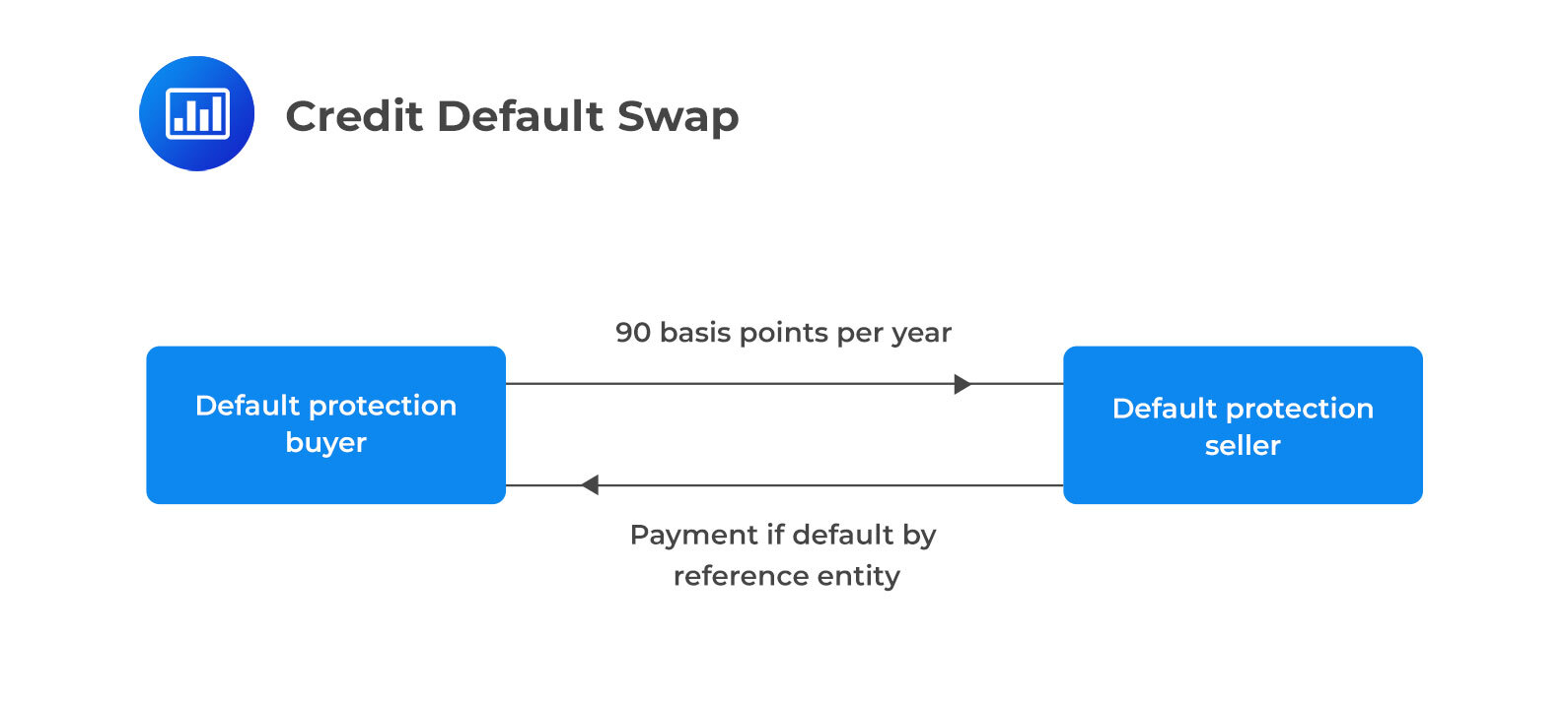
A Credit Default Swap (CDS) is the most prevalent form of single-name credit derivative where the underlying credit risk is associated with one specific entity. It operates similarly to an insurance policy against the default risk of the so-called ‘reference entity’ which can be a company or a country.

In a CDS transaction the buyer pays regular premiums to the seller in exchange for a commitment from the seller to compensate the buyer if the reference entity experiences a ‘credit event’ such as a default. ‘Physical settlement’ involves the transfer of defaulted bonds from the buyer to the seller who pays the par value in return whereas ‘cash settlement’ involves a financial payment based on the loss in value of the defaulted bonds as determined through an auction process.

Basket CDS

Basket CDS is a type of CDC that involves several reference entities. They come in different forms depending on the payout trigger:

• Add-up Basket CDS: Pays out when any of the reference entities default.
• First-to-Default CDS: Pays out only upon the first default in the basket.
• Second-to-Default CDS: Pays out only upon the second default and so on.

The payout is calculated similarly to a regular CDS and once the relevant default occurs and is settled the swap terminates with no further payments.

Total Return Swap (TRS)

A TRS is an agreement to exchange the total return on a bond or asset portfolio for a floating rate plus a spread encompassing coupons, interest, and any capital gains or losses.

Example: In a 5-year TRS with a notional principal of $100 million, the payer would exchange the total return on a corporate bond for a floating rate plus 25 basis points. At the end of the swap, a payment reflects the bond’s value change, with the payer or receiver compensating for any increase or decrease in value.

If the bond defaults, the swap typically ends and the receiver compensates for the difference between the notional principal and the bond’s market value. TRS can be a tool for transferring credit risk or taking a synthetic position in the bond.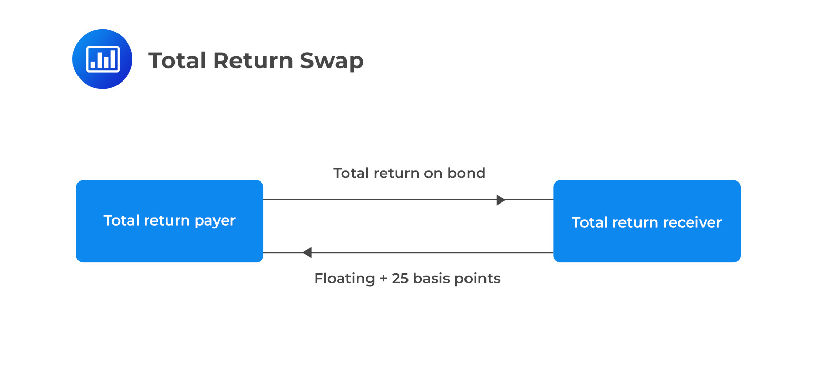

Collateralized Debt Obligations (CDOs)

CDOs are a type of asset-backed security where the underlying assets are bonds. They have a structured waterfall for interest and principal payments, ensuring senior tranches have priority over junior ones. There are two main types:

• Cash CDOs: These involve actual bonds as underlying assets.
• Synthetic CDOs: These use a portfolio of CDS contracts as underlying assets, selling protection on a chosen portfolio of companies. The principal of a synthetic CDO is the total notional of the underlying CDSs.

Synthetic CDOs distribute cash inflows from CDS spreads and outflows from defaults across different tranches according to predefined rules.

The market utilizes standardized portfolios like those underlying the CDX NA IG and iTraxx Europe indices to define standard synthetic CDO tranches. These can be traded actively without creating an underlying portfolio. The concept of single-tranche trading allows for trading one tranche independently of others

Accounting for Credit Risk in Valuing a CDS

Estimating Default Probabilities with Hazard Rates

Central to the valuation methodology is the ongoing hazard rate, which reflects the risk of default of the reference entity expressed as a continuously compounded rate. By establishing this rate, survival probabilities can be computed, representing the chances that the reference entity will avoid defaulting up until a certain time point. This involves exponential functions based on the hazard rate offering insights into the viability of the entity throughout the term of the CDS.

Assume the constant hazard rate for our reference entity is \(1.5\%\) per annum throughout the 5-year duration of the CDS. Using this hazard rate, we calculate survival probabilities with the formula:

\[ \text{Survival Probability} = e^{-\text{hazard rate} \times \text{time}} \]

Considering a hazard rate of \(1.5\%\) per annum, we can create the following table:

\[ \begin{array}{c|c|c} \textbf{Year} & \textbf{Probability of Surviving to Year End} & \textbf{Probability of Default During Year} \\ \hline 1 & e^{-0.015 \times 1} = 0.9851 & 0.0149 \\ 2 & e^{-0.015 \times 2} = 0.9704 & 0.0147 \\ 3 & e^{-0.015 \times 3} = 0.9559 & 0.0145 \\ 4 & e^{-0.015 \times 4} = 0.9416 & 0.0143 \\ 5 & e^{-0.015 \times 5} = 0.9275 & 0.0141 \\ \end{array} \]

The default probability in the third year, for example, is \(0.9704 – 0.9559 = 0.0145\).

Determining Payment Expectations in the Event of Default

Payments on the CDS are assumed to occur annually, with defaults anticipated to happen mid-year. The risk-free interest rate is set at \(3\%\) per annum with continuous compounding, and the recovery rate is \(50\%\). We calculate the present value of expected CDS payments assuming a payment rate of ‘s’ per year and a notional principal of $1.

$$\begin{array}{|c|c|c|c|}
\hline \textbf{Year}& \textbf{Probability of Payment} & \textbf{Expected Payment} & \textbf{Present Value of Payment}\\
\hline 1 & 0.9851 & 0.9851 \mathrm{s}& 0.9851 \mathrm{s} * \mathrm{e}^{-0.03 * 1} \\ \hline 2 & 0.9704 & 0.9704 \mathrm{s} & 0.9704 \mathrm{s} * \mathrm{e}^{-0.03 * 2} \\ \hline\ldots & \ldots& \ldots \\ \hline \end{array}$$

The sum of these present values gives us the total present value of the expected payments.

Expected Payoff Calculation

The expected payoff in the event of default is determined by the product of the default probability, the notional amount minus recovery, and the discount factor. The total present value of expected payoffs is calculated by summing these values.

$$\begin{array}{|c|c|c|c|}
\hline \textbf{Year} & \textbf{Probability of Default}& \textbf{Expected Payoff} & \textbf{Present Value of Payoff} \\
\hline 1 & 0.0149 & 0.0149 * 0.5 & 0.00745 * \mathrm{e}^{-0.03 * 0.5}\\
\hline 2 & 0.0147 & 0.0147 * 0.5 & 0.00735 * \mathrm{e}^{-0.03 * 1.5}\\
\hline \ldots & \ldots & \ldots & \ldots \\ \hline \end{array}$$

Finally, to find the CDS spread ‘s,’ equate the present value of expected payoffs with the present value of expected payments. Solving for ‘s’ gives the annual spread that would make the CDS fair-priced.

Determining the CDS Spread

Finally, to find the CDS spread ‘s,’ equate the present value of expected payoffs with the present value of expected payments. Solving for ‘s’ gives the annual spread that would make the CDS fair-priced.

Incorporating the Recovery Rate

The recovery rate, commonly set at a standard value like 40%, is factored into the valuation process to represent the anticipated percentage recovery of the bond’s face value immediately post-default. By integrating the probability of default and the cost of protection into the valuation, financial professionals can derive a sophisticated understanding of the CDS’s value. This careful accounting for credit risk ensures that potential losses due to credit risk over the life of the CDS are encapsulated in the valuation, allowing for an accurate reflection of the instrument’s worth and risk exposure.

Default Probabilities for CDS Valuation

In the valuation of Credit Default Swaps (CDS), pinpointing default probabilities is vital for determining both the price and expected payments related to the protection provided by the swap.

Index CDS as a Benchmark for Default Probabilities

An Index CDS encompasses a basket of single-name reference entities and thus offers insights into the average default probability across a diverse set of entities. By taking reference from an Index CDS, traders can understand the average market expectation of credit risk, which is a starting point for estimating individual default probabilities.

Quoted Spreads and Hazard Rates

When dealing with single-name CDS or Index CDS, quoted spreads provide the initial perception of credit risk. However, for an accurate valuation, traders imply hazard rates from these quoted spreads. The hazard rate effectively captures the risk of default annually and is fundamental for the valuation of CDS instruments.

Implicit calculations in valuation

Valuations involve “implying” a hazard rate from the quoted spread through iterative calculations. This process requires a recurring estimation that aligns the market spread with the probabilistic model of default underpinning the CDS valuation. The result is an implied risk profile that serves as a more precise measure of default probability.

Duration and Price Determination

The concept of “duration” in the context of CDS valuation is instrumental, though it differs from traditional fixed income duration. In this scenario, duration represents a factor by which the quoted spread is adjusted to arrive at the present value of expected spread payments throughout the CDS life. The price, in turn, hinges upon this duration and the difference between the quoted spread and the fixed coupon rate.

By establishing rigorous methods to identify default probabilities, practitioners can provide a more nuanced and market-reflective valuation for CDS. This involves not just a static view of credit risk but an adaptable approach that accommodates fluctuations in market perceptions and conditions over time. It’s this comprehensive risk measurement that ensures credit derivatives are traded at prices that accurately reflect the underlying credit risk.

Evaluating Credit Indices and Fixed Coupons in CDS Pricing

When determining the pricing of Credit Default Swap (CDS) contracts, credit indices, and fixed coupons play a significant role in streamlining transactions and reflecting aggregated risk perceptions.

Credit Indices as Indicators of Default Risk

Credit indices are used to monitor CDS spreads. Significant indices include:

• CDX NA IG: Encompasses 125 top-tier companies in North America.
• iTraxx Europe: Contains 125 prime investment-grade entities in Europe.

These indices are updated biannually, with adjustments made to include or exclude companies based on their investment grade status. The cost of buying CDS protection is represented by the index spread.

Example of Credit Index Pricing:

For instance, the 5-year iTraxx Europe index might be quoted at 75 basis points bid and 76 basis points ask per unit of notional value. This indicates the rate at which protection can be bought for the index’s entire portfolio of companies.

Credit indices, such as CDX NA IG and iTraxx Europe, compile a basket of single-name CDS to assess the overall credit risk of a group of reference entities. These indices simplify the process of gauging default probabilities across a broader market segment, thereby assisting in pricing CDS contracts. They serve as benchmarks for the credit market and offer a standardized way to trade credit risk.

The Role of Fixed Coupons in CDS Transactions

Fixed coupons standardize the payments in CDS transactions. In contrast to fluctuating spreads, a fixed coupon simplifies the trading process by setting a uniform payment rate for protection sellers. This fixed rate is determined in relation to prevailing market spreads and typically gets adjusted at regular intervals, such as every quarter, to stay aligned with current credit conditions.

Credit Default Swap (CDS) and CDS index transactions are more intricate than one might initially perceive. In these transactions, a fixed coupon and a specific recovery rate are predetermined for each underlying asset and its corresponding maturity. The price of the CDS is then derived from the quoted spread through a multi-step process:

1. Quarterly Payments Assumption: It is assumed that payments are made four times a year in arrears.
2. Hazard Rate Implication: The hazard rate is deduced from the quoted spread via an iterative calculation process. This rate reflects the probability that the reference entity will experience a credit event, and it is integral to determining the price of the CDS.
3. Duration Calculation: A duration, represented by ‘D,’ is calculated for the CDS payments. This duration acts as a multiplier for the spread to determine the present value of spread payments.
4. Price Determination: The price ‘P’ is given by the formula

$$
P=100-100 \times D \times(s-c)
$$

where ‘ \(s\) ‘ is the spread and ‘c’ is the coupon, both expressed in decimal form.

When a trader purchases protection, they pay 100 – P per \(\$ 100\) of the total remaining notional amount, and conversely, the seller of protection receives this amount. The buyer then makes regular quarterly payments based on the coupon rate and the remaining notional value, which is adjusted if there are any defaults in the underlying names.

Example Illustration

Let’s consider an example using the iTraxx Europe index as a reference point:

• Suppose the quoted index is 36 basis points, and the coupon is 50 basis points for a 5-year contract.
• The yield curve is assumed to be flat at \(2 \%\) per annum, with continuous compounding and a recovery rate of \(45 \%\).
• Four payments are made per year, with the implied hazard rate calculated to be \(0.59 \%\).
• The duration ‘ \(\mathrm{D}\) ‘ is found to be 4.5 years.

The price ‘P’ would thus be calculated as:

$$
P=100-100 \times 4.5 \times(0.0036-0.0050)=101.4
$$

In a scenario where the protection covers \(\$ 2\) million per entity, initially, the seller of protection would pay the buyer \(\$ 2,000,000 \times 125 \times 0.014\). Subsequent quarterly payments by the buyer would be at an annual rate of \(\$ 2,000,000 \times 0.0050 \times n\), where ‘ \(n\) ‘ is the number of entities that have not experienced default.

The CDS market spread serves as a dynamic proxy for the default risk of the underlying entities. This spread varies according to market sentiment regarding the likelihood of default. For valuation purposes, the current market spread must be adjusted by a factor related to duration, which diverges from traditional fixed-income duration concepts. The adjusted spread then influences the pricing by reflecting the present value of expected spread payments over the CDS lifespan.

CDS-Bond Basis

The CDS-bond basis is a critical metric in the credit derivatives market, calculated as:

$$
\text { CDS bond basis }=\text { CDS spread }- \text { Bond yield spread }
$$

This formula serves to compare the CDS spread against the yield spread of a comparable bond. It is a vital tool for relative value analysis in the credit market, offering insights into the discrepancy between the perceived credit risk of a bond and a CDS on the same reference entity.

Example: Calculation of CDS-Bond Basis

Consider a scenario where the CDS spread for a specific entity is 150 basis points, and the bond yield spread over a similar risk-free rate is 100 basis points. The CDS-bond basis, in this case, would be:

$$
150 \mathrm{bps}-100 \mathrm{bps}=50 \mathrm{bps}
$$

This 50 bps CDS-bond basis indicates the relative pricing difference between the CDS and the bond. A positive basis suggests that the market perceives the CDS as more expensive relative to the bond, potentially reflecting higher credit risk or other market dynamics such as liquidity premiums.

The CDS-bond basis fluctuates with market conditions, offering insights into investor sentiment and credit market trends. A widening basis can signal increasing caution among investors, while a narrowing basis might indicate growing confidence in the creditworthiness of the reference entity.

CDS Forwards and CDS Options

Valuation and trading strategies for Credit Default Swaps (CDS) are augmented by the utilization of forwards and options structured around CDS contracts, providing tailored risk management and speculative opportunities.

Credit Default Swap Forwards (CDS Forwards)

A CDS forward is an agreement to enter into a CDS contract at a specified future date at an agreed-upon fixed spread. The buyer of a CDS forward is obligated to become the protection buyer, and the seller is obligated to become the protection seller at a future point in time. The essential feature of a forward contract is that it locks in the current spread for future protection, offering a hedge against potential worsening credit conditions of the reference entity.

Credit Default Swap Options (CDS Options)

CDS options, or options on CDS (often called CDS swaptions), grant the holder the right but not the obligation to enter a CDS contract at a specific spread (the strike). Like other options, CDS options are categorized as “calls” and “puts”:

• A CDS call option gives the purchaser the right to buy protection (to become the protection buyer in a CDS) at a predetermined spread, which is useful if the purchaser anticipates credit deterioration.
• A CDS put option allows the holder to sell protection (to become the protection seller in a CDS) at a predetermined spread, suitable if the holder expects credit improvement.

The underlying spread at which the buyer of a call or seller of a put can transact is the strike of the option. Counterparties use these instruments to manage uncertainty and to speculate on the credit quality of reference entities without the immediate commitment of entering into a CDS contract.

Valuing a Synthetic CDO Using Spread Payments and Gaussian Copula Models

Valuing a Synthetic Collateralized Debt Obligation (CDO) is an intricate process involving modeling the timing and likelihood of defaults across a portfolio of reference entities. Two popular approaches for this valuation are the spread payments and the Gaussian copula models.

Spread Payments Approach

The spread payments approach calculates the value of a synthetic CDO tranche by determining the expected payments to be made on the CDS contracts that make up the reference portfolio of the CDO. These payments include periodic protection premiums
and potential payouts upon default events. The valuation considers the present value of the expected spread payments against the likelihood of defaulting counterparties in the reference portfolio, along with the loss-given default affecting the tranche in question.

Gaussian Copula Model of Time to Default

The Gaussian copula model is a sophisticated mathematical framework that relates the default times of different entities. It assumes a single factor that influences all entities within a portfolio and computes the joint probability of default by incorporating correlations among the entities. This one-factor model has become a market standard for pricing both single-tranche CDS and synthetic CDOs due to its relative simplicity and the ability to capture the default dependence structure across entities.

Valuation of kth-to-Default CDS

In a kth-to-default Credit Default Swap (CDS), the valuation process seeks to determine the price at which the CDS should be traded, given the probability of the kth default within a portfolio of reference entities.

Calculating the kth Default Probability

The key to valuing a kth-to-default CDS is to calculate the probability that exactly \(\mathrm{k}\) defaults occur by a certain time, which can be expressed using the binomial distribution. This probability depends on the systemic factor \(\mathrm{F}\) and is calculated by:

$$
\mathrm{P}(\mathrm{k}, \mathrm{tj} \mid \mathrm{F})=\left(\begin{array}{l}
\mathrm{n} \\
\mathrm{k}
\end{array}\right) \mathrm{Q}\left(\mathrm{t}_{\mathrm{j}} \mid \mathrm{F}\right)^{\mathrm{k}}\left(1-\mathrm{Q}\left(\mathrm{t}_{\mathrm{j}} \mid \mathrm{F}\right)\right)^{\mathrm{n}-\mathrm{k}}
$$

Where:

• \(\mathrm{n}\) is the total number of entities in the portfolio.
• \(\mathrm{Q}(\mathrm{t} \mid \mathrm{F})\) is the conditional probability of default by time \(\mathrm{t}\), given \(\mathrm{F}\).

Example:

Let’s consider a simplified example for a fourth-to-default CDS on a portfolio of 12 reference entities:

• Assume each entity has a hazard rate of \(1.5 \%\) per annum.
• Suppose the copula correlation is 0.2.
• The recovery rate is \(50 \%\).
• All risk-free rates are at \(3.5\%\).

If the time intervals for payment dates are annual and in arrears, we need to compute the expected tranche principal and payments for each period.

Using the Gaussian Copula Model of Time to Default

The Gaussian copula model facilitates the joint modeling of default times by assuming a standard normal distribution for the systemic factor \(\mathrm{F}\).

For a given time \(\mathrm{t}\) and a standard normal variable \(\mathrm{F}\), the conditional probability of default is determined using the formula:
$$
\mathrm{Q}(\mathrm{t} \mid \mathrm{F})=\Phi\left(\frac{\left(\Phi^{-1}(\mathrm{Q}(\mathrm{t}))-\sqrt{\rho \mathrm{F})}\right.}{\sqrt{1-\rho}}\right)
$$
where \(\Phi\) denotes the cumulative distribution function of the standard normal distribution, \(\rho\) is the copula correlation, and \(Q(t)\) is the unconditional probability of default by time \(t\), calculated from the hazard rate \(h\) as \(Q(t)=1-e^{-h t}\).

Example: Using the Gaussian Copula Model
For our example portfolio of 12 bonds, we can apply the Gaussian copula model to calculate the present value of expected payments and payoffs. The computation involves numerical integration over the distribution of \(\mathrm{F}\), typically using Gaussian quadrature for accuracy.

Let’s say we wish to value the tranche for a period of 5 years, with payments made annually. Using Gaussian quadrature with 20 integration points, we would calculate the present value of payments and payoffs at each time interval, taking into account the correlation among defaults.

Let’s create an example based on the methodology for valuing a kth-to-default CDS using a Gaussian Copula Model. We’ll do this for a third-to-default CDS.

Example: A Third-to-Default CDS Valuation

For our portfolio, we will consider:

• Number of bonds ( \(\mathrm{n}): 10\)
• Hazard rate \((\mathrm{h})\) for each bond: \(2 \%\)
• Copula correlation \((\rho): 0.3\)
• Recovery rate \((\mathrm{R}): 40 \%\)
• Risk-free rate: \(5 %\)

We will value the CDS at annual intervals over 5 years.
Step 2: Calculate Unconditional Default Probabilities
Unconditional default probability for each year using the hazard rate:

$$
Q(\mathrm{t})=1-\mathrm{e}^{-\mathrm{ht}}
$$

For \(\mathrm{t}=1\) to 5 years with \(h=0.02\) :
$$\begin{aligned}
& \mathrm{Q}(1)=1-\mathrm{e}^{-0.02 \times 1} \approx 0.0198 \\
& \mathrm{Q}(2)=1-\mathrm{e}^{-0.02 \times 2} \approx 0.0392 \\
& \mathrm{Q}(3)=1-\mathrm{e}^{-0.02 \times 3} \approx 0.0582 \\
& \mathrm{Q}(4)=1-\mathrm{e}^{-0.02 \times 4} \approx 0.0769 \\
& \mathrm{Q}(5)=1-\mathrm{e}^{-0.02 \times 5} \approx 0.0952
\end{aligned}$$

Step 3: Calculate Conditional Default Probabilities
Using the Gaussian Copula Model and assuming a standard normal distribution for the systemic factor \(F\), calculate the conditional default probability:
$$
Q(t \mid F)=\Phi\left(\frac{\left(\Phi^{-1}(Q(t))-\sqrt{\rho F}\right)}{\sqrt{1-\rho}}\right)
$$

This step involves numerical methods to compute \(\Phi^{-1}\) and \(\Phi\), which are the inverse cumulative distribution function and the cumulative distribution function of the standard normal distribution, respectively.

Step 4: Calculate the Present Value of Expected Payments and Payoffs
We assume defaults occur at the midpoint of each interval \(\left(0.5 t_j-1+0.5 t_j\right)\). The present value of expected payments is calculated assuming a spread ‘s’ paid annually:
$$
\operatorname{PV} \text { (payments) }=\sum_{\mathrm{j}=1}^5 \mathrm{~s} \times \mathrm{Q}\left(\mathrm{t}_{\mathrm{j}} \mid \mathrm{F}\right) \times \mathrm{e}^{-0.05 \times \mathrm{t}_{\mathrm{j}}}
$$

The present value of expected payoffs, assuming default occurs halfway through each year:
$$
\mathrm{PV}(\text { payoffs })=\sum_{\mathrm{j}=1}^5(1-\mathrm{R}) \times\left(\mathrm{Q}\left(\mathrm{t}_{\mathrm{j}}-1 \mid \mathrm{F}\right)-\mathrm{Q}\left(\mathrm{t}_{\mathrm{j}} \mid \mathrm{F}\right)\right) \times \mathrm{e}^{-0.05} \times\left(0.5 \mathrm{t}_{\mathrm{j}-1}+0.5 \mathrm{t}_{\mathrm{j}}\right)
$$

Step 5: Calculate the Break-even Spread

The break-even spread ‘s’ is the spread that equates the present value of expected payments with the present value of expected payoffs:
$$
s=\sum j=\frac{P V(\text { payoffs })}{\sum_{j=1}^5 Q\left(t_j \mid F\right) \times e^{-0.05 \times t_j}}
$$

Application to CDO Tranches

When applied to CDO tranches, the Gaussian copula model facilitates the computation of expected losses and values for different tranches of debt, categorized according to their risk levels, such as senior, mezzanine, and equity tranches. Valuations derived from these models are core to trading and risk assessment functions in the credit derivatives market.

Understanding Implied Correlation in CDO Valuation

Implied correlation is a pivotal concept in the valuation of collateralized debt obligations (CDOs), specifically in regards to the dependencies between default events in a CDO tranche’s underlying assets.

Compound (Tranche) Correlation

Compound or tranche correlation is derived from the market prices of tranches and refers to the correlation assumption needed to match model prices with market prices. It’s a single correlation figure for each tranche that, when input into a pricing model such as the Gaussian copula, reproduces the market-observed price of the tranche. This type of correlation measures the implied average dependency between defaults within a portfolio and serves as an important gauge for investors to understand the risks associated with different tranches. However, it is a simplification as it does not differentiate between individual correlations of reference entities.

Base Correlation

Base correlation represents an approach to deal with the inconsistencies found in compound correlation across different tranches. These correlations reflect the market’s view of dependence at different attachment and detachment points of a CDO’s capital structure. In practice, base correlations are used to calculate expected losses on tranches, but they can yield non-arbitrage problems when interpolated. To address this, a direct interpolation of expected losses, instead of base correlations, can provide a better estimation of tranche losses and satisfy no-arbitrage conditions.

Interpolating Expected Losses

Instead of relying solely on base correlations, which can lead to arbitrage opportunities, the industry has moved towards directly interpolating expected losses across different attachment points in a CDO tranche structure. This approach ensures that expected losses increase at a decelerating rate and satisfy no-arbitrage conditions, providing a more stable and accurate gauge for determining the tranche’s value in the context of overall portfolio risk.

Implied correlation, whether tranche or base, is a complex measure that provides insight into how the market values the interconnectedness of default risk in CDOs. The utilization of direct expected loss interpolation further refines the valuation process and offers a mechanism that more accurately reflects the risks inherent in these structured credit instruments. Understanding the nuances of implied correlation and the associated valuation techniques equips financial risk managers with the analytical tools necessary to assess and manage the risks presented by CDOs.

Alternative Approaches to Estimate Default Correlation

Estimating default correlation is a critical component of credit risk management, particularly when assessing the potential for simultaneous defaults in portfolios of credit-sensitive assets. Several alternative approaches to the standard market models provide diverse perspectives on correlation and default risk.

Heterogeneous Models

A step beyond the commonly used homogeneous models, which imply identical time-to-default probability distributions and equal copula correlations for all entities, is the use of heterogeneous models. These models allow for differences in default probabilities and correlations across various entities. This leads to a more sophisticated and accurate representation of default risks but also complicates the model’s implementation because default probabilities are individualized and cannot simply rely on broad formulas. This necessitates the use of numerical procedures for valuation.

Alternative Copula Models

One-factor Gaussian copula is a standard in modeling correlation between default times, but numerous alternatives exist, such as the Student t copula, Clayton copula, Archimedean copula, and Marshall–Olkin copula. These models vary in assumptions and complexity. Models incorporating non-normal distributions for factors, such as the double t copula proposed by Hull and White, have proven effective at fitting market data. Moreover, introducing additional factors into these models allows for even higher fidelity in representing default correlations, though it substantially increases computational demands.

Random Recovery and Factor Loadings

Models suggested by Andersen and Sidenius introduce variations in the copula correlation, making it a function of economic factors, and suggest a negative relationship between recovery rates and default rates. These nuanced approaches reflect empirical observations that defaults tend to be more highly correlated during times of economic stress, thereby improving model accuracy and market fit.

The Implied Copula Approach

Analogous to the concept of implied volatility in equity options, the implied copula approach seeks to determine a copula from market quotes. This model often assumes average hazard rates for all companies within a portfolio and derives probability distributions for these hazard rates from the market prices of tranches.

Dynamic Models

Dynamic models contrast with the static frameworks typically employed for CDO valuation. They model the evolution of portfolio loss through time and may include structural models that simulate asset prices for multiple companies, reduced-form models focusing on hazard rates and their jumps, and top-down models that directly model portfolio loss without dissecting individual company performance.

In sum, these varied methodologies for estimating default correlation challenge and enhance the conventional one-factor Gaussian copula model. By considering different model structures and introducing more refined assumptions about default dependencies, market participants can achieve a better alignment with empirical evidence and market behavior, ultimately leading to more accurate pricing and risk assessment of credit derivatives.

Practice Question

Consider a CDS contract on a single reference entity where the market spread is 200 basis points, and the fixed coupon is set at 100 basis points. Assume the credit curve is flat, with continuous compounding at an annual risk-free rate of 2% and a recovery rate of 40%. Quarterly payments are agreed upon in the contract, and the CDS duration calculated for the payments is determined to be 4.8 years. As an FRM candidate, can you calculate the initial upfront payment per $100 of notional that the protection buyer must pay to the protection seller?

1. $105.92
2. $108.16
3. $95.20
4. $94.08

The correct answer is C.

The price \( P \) of a CDS contract can be determined using the formula \( P=100-100 \times D \times (s-c) \), where \( s \) is the spread, \( c \) is the coupon, and \( D \) is the duration of the contract payments, all expressed in decimal form. In this case, \( s=0.0200 \), \( c=0.0100 \), and \( D=4.8 \) years. Plugging these values into the formula, \( P=100-100 \times 4.8 \times (0.0200-0.0100) \).

Performing this calculation:

\( P=100-100 \times 4.8 \times 0.0100 \)

\( P=100-4.8 \times 1 \)

\( P=100-4.8 \)

\( P=95.2 \)

Therefore, the protection buyer must pay the protection seller an initial upfront payment of $95.20 per $100 of notional. 

A is incorrect because a price of $105.92 would suggest the spread is lower than the coupon, which contradicts the given information.

B is incorrect because a price of $108.16 suggests an even greater disparity opposite to the provided spread and coupon relationship.

D is incorrect because a price of $94.08 underestimates the impact of the spread and coupon difference in the CDS pricing formula.

Things to Remember

• The upfront CDS payment is effectively a price adjustment that reflects the difference between the market spread and the fixed coupon, discounted over the duration at the risk-free rate.
• Understanding the formula for calculating the price of a CDS is critical in pricing and risk management, as it incorporates key elements such as the spread, coupon, duration, and recovery rates.