


Balance Sheet Modeling

The basic fundamental law of active portfolio management states that the optimal expected active return is the product of the assumed information coefficient (IC), the square root of breadth (BR), and the active portfolio risk.
The ex-ante information ratio of a manager is built on two factors i.e., skill, and breadth. Skill is gauged by the information coefficient (IC) or the correlation between the expected return and the actual return. Note that IC is assumed to be identical for all estimates. Further, remember that breadth (BR) is the number of independent estimates of exceptional returns made at a given frequency in a year.
The information ratio of an unconstrained optimal portfolio is therefore given by:
$$ IR^\ast=IC\times\sqrt{BR} $$
The expected value added by active management is given by:
$$ E\left(R_A\right)^\ast=IC\times\sqrt{BR}\times\sigma_A $$
The IC ranges between -1 and 1. A perfectly brilliant manager has an IC of 1, while a perfectly wrong manager has an IC of -1. A manager with no skill, on the other hand, has an IC of 0. Moreover, a portfolio will be more efficient when the breadth of the bets (estimates) is higher.
The fundamental law of active management assumes that a portfolio manager accurately measures the value of their information and subsequently builds portfolios that optimally use that information.
It is worth remembering that the basic law of active management (Grinold’s fundamental law) calculates the information ratio (IR) as the product of the assumed information coefficient (IC) and the square root of breadth (BR). However, the theoretically calculated value of IR overestimates the IR that a manager can reach.
For example, if the monthly information coefficient (IC) is 0.04 and the selection universe is 1,050 stocks, the expected annualized IR is:
$$ =0.04\times\sqrt{12\times1050}=4.49 $$
An IR of 4.49 is even above the most optimistic manager’s dreams.
To reduce the high information ratio, a third term called the transfer coefficient (TC) can be added to the information ratio equation. It is defined as the correlation between the forecasted active returns and the actual active weights of a portfolio. It measures the efficiency with which a manager translates their insights into their portfolio bets.
The transfer coefficient ranges from -1 to +1. An unconstrained portfolio has a TC of 1. This implies that the actual active weights are equal to the forecasted active returns, allowing the full expected value added to be reflected in the portfolio structure. The TC will be less than 1 for a portfolio with imposed constraints such as active risk.
$$ TC=CORR\left(\frac {\mu_i}{\sigma_i},\Delta w_i \sigma_i\right)=CORR \left(\Delta w_i×\sigma_i,\Delta w_i \sigma_i \right) $$
Where:
Incorporating the impact of the transfer coefficient, the full fundamental law can be expressed in the following equation:
$$ E\left(R_A\right)=TC\times IC\times\sqrt{BR}\times\sigma_A $$
And
$$ IR=TC\times IC \times\sqrt {BR} $$
Brad Cooper is a portfolio manager at Penn Investment Limited. Cooper manages a portfolio of four securities, and his goal is to gauge the expected portfolio return. The following is information relating to the four securities:
$$ \begin{array}{c|c|c|c} \textbf{Security} & \textbf{Expected Active} & \textbf{Active Return} & \textbf{Actual active} \\ {} & \textbf{Return} & \textbf{Volatility } \bf{({\sigma}_{i})} & \bf{\text{weight } ({w}_{i})} \\ \hline A & 0.39\% & 1.97\% & 7.00\% \\ \hline B & 0.79\% & 3.93\% & 5.00\% \\ \hline C & -0.39\% & 1.97\% & 8.00\% \\ \hline D & -0.89\% & 3.93\% & -30.00\% \end{array} $$
Further, Cooper has generated the following components using an automated excel spreadsheet:
\(Cov \left(\frac{\mu_i}{\sigma_i}, \Delta w_i \sigma_i\right)= 0.074\%\)
\(Var \left(\Delta w_i \sigma_i \right)= 0.0033916{(\%^2)}\)
\(Var \left(\frac{\mu_i}{\sigma_i} \right) = 4.266{(\%^2)}\)
Note: The units on variance are the square of the units of the underlying data.
Use the above information to calculate:
$$ TC=CORR\left(\frac {\mu_i}{\sigma_i},\Delta w_i \sigma_i\right) $$
Note that:
$$ \begin{align*} CORR \left(X,Y\right) &=\frac{COV\left(XY\right)}{\sigma_X\sigma_Y} \\ TC & =\frac{0.074\%}{\sqrt{4.266{(\%}^2)}\times\sqrt{0.0033916{(\%^2)}}}=0.6152 \end{align*} $$
$$ \begin{align*} E\left(R_A\right) &=TC\times IC\times\sqrt{BR}\times\sigma_A \\ & =0.6152\times0.75\times\sqrt9\times10=13.84\% \end{align*} $$
In the previous section, we learnt that the optimal amount of active risk of an unconstrained portfolio is given by:
$$ \sigma_P^\ast=\frac{IR}{SR_B}\times\sigma_B $$
The transfer coefficient is applicable in the calculation of the optimal level of active risk for a constrained, actively managed portfolio. The optimal amount of active risk is given by:
$$ \sigma_A=TC\times\frac{IR^\ast}{SR_B}\sigma_B $$
Where \({IR}^\ast\) is the information ratio of an unconstrained portfolio. This leads to a maximum value of the squared Sharpe ratio of a constrained portfolio:
$$ SR_P^2=SR_B^2+\left(TC\right)^2\left(IR^\ast\right)^2 $$
Note that with a transfer coefficient of 0, the optimal level of active risk becomes 0. This implies that the manager should invest solely in the benchmark portfolio.
So far, the fundamental law relates to the expected value added through active portfolio management. Nevertheless, the actual performance can differ from the expected value in a range that can be determined by active risk.
We can measure the actual performance of a portfolio by establishing the relationship between realized relative returns and relative weights. Given the ex-post realized information coefficient \((IC_R)\), the fundamental law of active management can be expressed as:
$$ E\left(R_A\middle| I C_R\right)=TC\times IC_R\times\sqrt{BR}\times\sigma_A $$
Where \(E\left(R_A\middle| I C_R\right)\) represents the expected value-added, given an investor’s realized skill.
The difference between the actual active portfolio return and the expected active portfolio return is replaced with a noise term.
That is:
$$ \text{Noise}=R_A-E\left(R_A\middle| IC_R\right) $$
Therefore, the actual active portfolio return is given by:
$$ R_A=E\left(R_A\middle| I C_R\right)+ \text{Noise} $$
Where \(R_A\) is the actual active return and \(E\left(R_A\middle| I C_R\right)\) represents the expected value-added, given an investor’s realized skill. The noise emerges from the impact of the constraints on the optimal portfolio.
The following chart illustrates the fundamental law of active management.
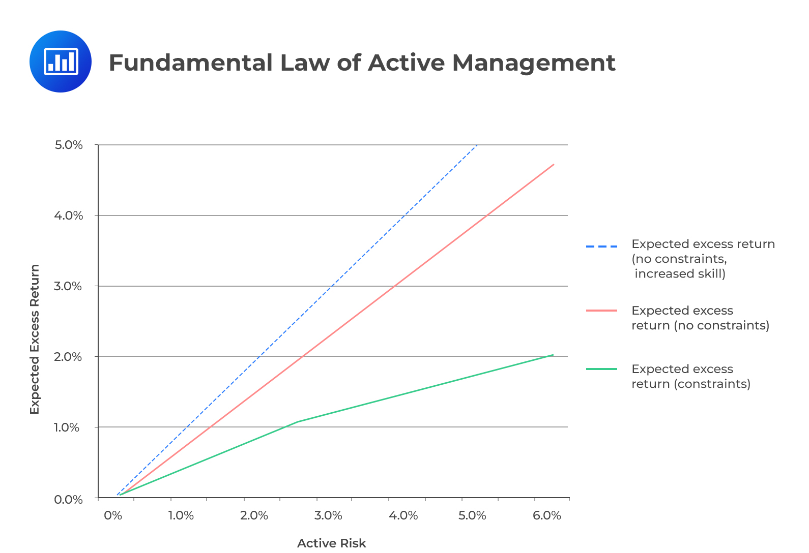 For a portfolio with no constraints, the trade‐off would be a straight line for a given level of skill. This means that the expected excess return relative to the index increases with the increase in a manager’s skills and active risk.
With the presence of constraints such as no short selling, sector limitations, and turnover limitations, the expected excess return would decrease for any given level of active risk. This is because the constraints would impair a manager’s ability to translate his or her information into the portfolio positions.
Question
An active management strategy includes ninety-six investment decisions, a realized information coefficient of 0.08, and a transfer coefficient of 0.90. The annualized active risk of the strategy is 5%, and the actual return on the active portfolio is 3.62%. The amount of forecasted active return that was offset by the noise component is closest to:
- 0.01%.
- 0.04%.
- 0.09%.
Solution
The correct answer is C.
$$ \begin{align*} E\left(R_A\right) & =TC\times IC\times\sqrt{BR}\times\sigma_A \\ E\left(R_A\right) &=0.9\times0.08\times\sqrt{96}\times5\%=3.53\% \end{align*} $$
Since
$$R_A=E\left(R_A\middle| I C_R\right)+ \text{Noise} $$
We have,
$$ \text{Noise}=R_A-E\left(R_A\middle| I C_R\right)=3.62\%-3.53\%=0.09\% $$
Reading 44: Analysis of Active Portfolio Management
LOS 44 (c) State and interpret the fundamental law of active portfolio management including its component terms—transfer coefficient, information coefficient, breadth, and active risk (aggressiveness).
The fundamental law of active portfolio management is an important CFA Level II Portfolio Management concept. Candidates may be tested on how skill, breadth, transfer coefficient, and active risk influence expected active returns and information ratios.
To strengthen your preparation, explore the CFA Level II study program with practice questions, mock exams, and guided lessons.
Offered by AnalystPrep


Get Ahead on Your Study Prep This Cyber Monday! Save 35% on all CFA® and FRM® Unlimited Packages. Use code CYBERMONDAY at checkout. Offer ends Dec 1st.