Assumptions Underlying Multiple Linear Regression

The following assumptions are used to build multiple regression models:

• The relationship between the dependent variable, and the independent variables, is linear.
• The independent variables are not random.
• There is no definite linear relationship between two or more independent variables. A high correlation between two or more independent variables is known as multicollinearity.
• The expected value of the error term, conditional on the independent variables, is equal to 0.
• The variance of the error term is equal for all observations. This is known as the homoskedasticity assumption.
• The error term is uncorrelated across all observations.
• The error term is normally distributed.

The following assumptions are investigated, and their outcomes are analyzed (if violated) as follows:

1. Linearity: The regression algorithm would mathematically fail to capture the trend when fitted to a nonlinear, non-additive data set.
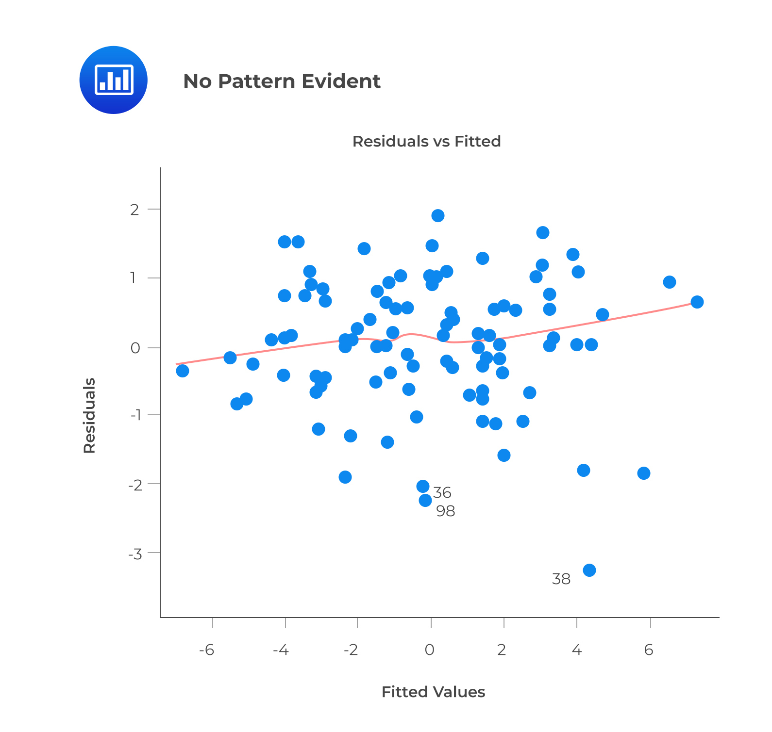   A prediction based on unobserved data will also be incorrect. The model can capture the nonlinear effect by including polynomial terms.

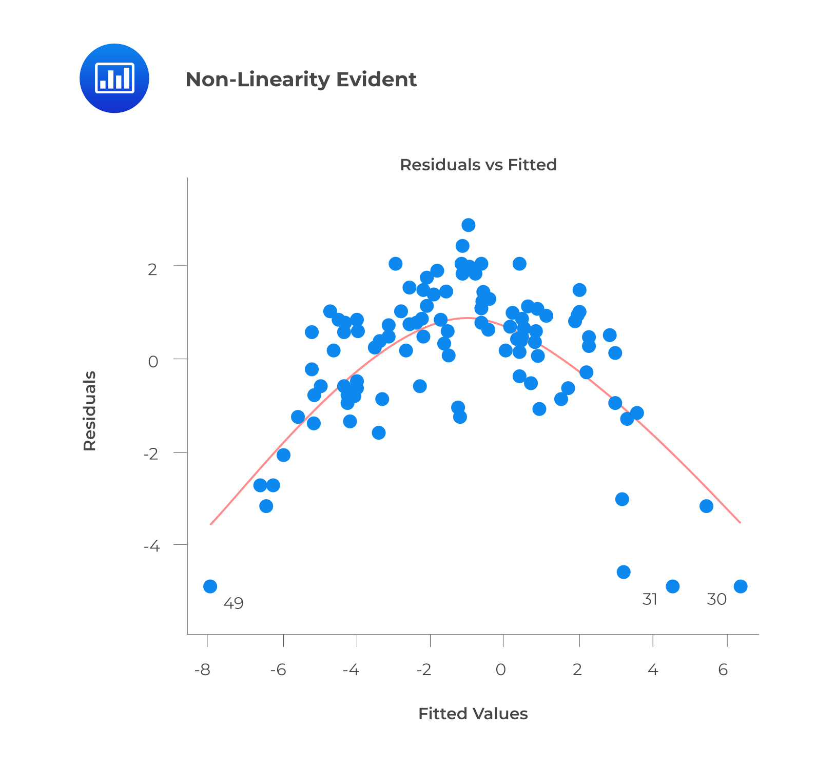
   This plot may show non-linearity if any pattern (such as a parabolic shape) appears. In other words, the model fails to capture nonlinear effects.

   

2. Autocorrelation: A model’s accuracy is drastically reduced when correlation exists in error terms. A time series model is characterized by this interaction, in which the next instant depends on the previous one.

   Correlated error terms tend to underestimate the true standard errors. Consequently, the estimated standard errors are likely higher than they should be. Note that confidence intervals and prediction intervals are narrowed if this occurs. The probability of the actual coefficient value being contained in a 95% confidence interval is lower than 0.95 if the confidence interval is narrower.

   To check for autocorrelation, calculate Durbin-Watson (DW) statistics. The value must be between 0 and 4. If DW = 2 implies no autocorrelation, \(0 < DW < 2\) implies positive autocorrelation, while \(2 < DW < 4\) indicates negative autocorrelation. The residual values can also be plotted against time to identify seasonal or correlated patterns.

3. Multicollinearity: A moderately or highly correlated set of independent variables will exhibit this phenomenon. In a model with correlated variables, it is challenging to determine the true relationship between a predictor and response variable.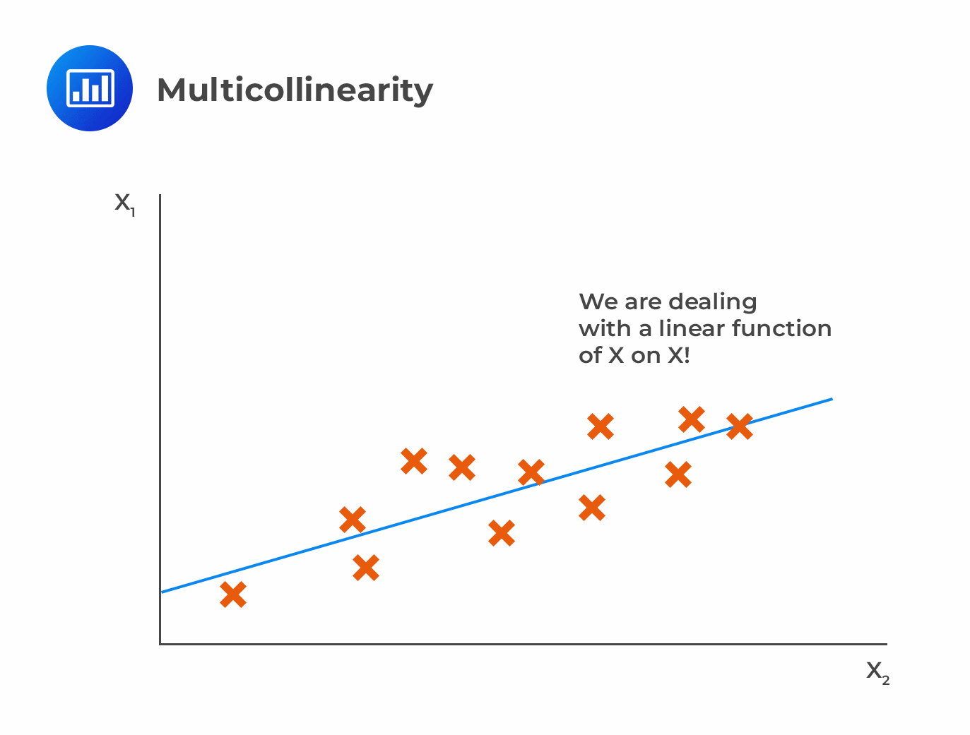

   The difficulty lies in determining which variable contributes to the response’s prediction. Furthermore, standard errors tend to increase when correlated predictors are present. A large standard error also leads to wider confidence intervals, resulting in less accurate slope parameters.

   Correlated predictors have a different regression coefficient depending on which other predictors are included in a model. A variable that strongly / weakly affects a target variable will result in an incorrect conclusion.

   Scatter plots can visualize correlations between variables to check for multicollinearity. VIF factor can also be used. VIF value <= 4 suggests no multicollinearity, whereas a value of >= 10 implies serious multicollinearity.

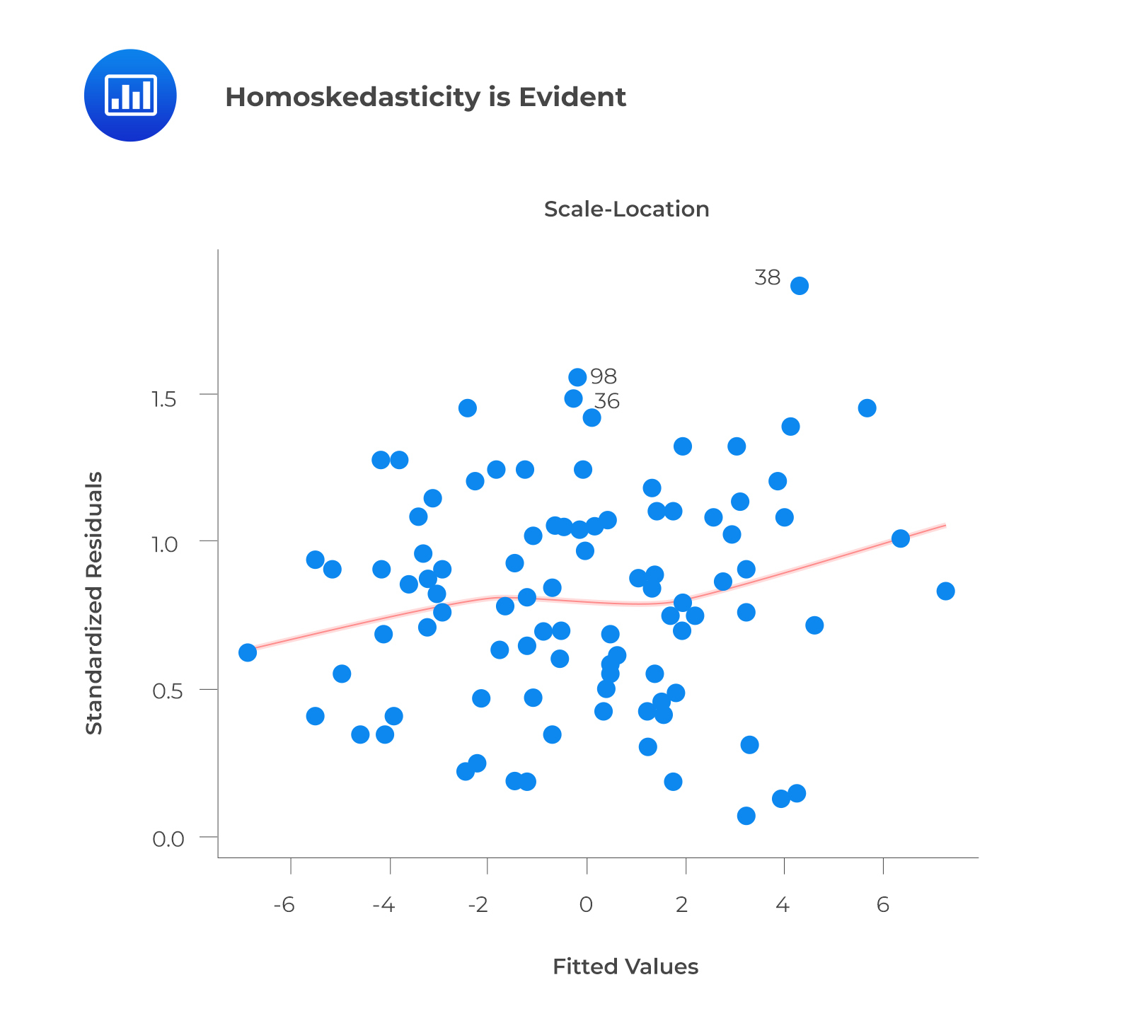
4. Heteroskedasticity: In heteroskedasticity, the error terms have non-constant variances.
   An outlier or extreme leverage value will typically lead to non-constant variance. These values disproportionately affect a model’s performance because they are given too much weight.

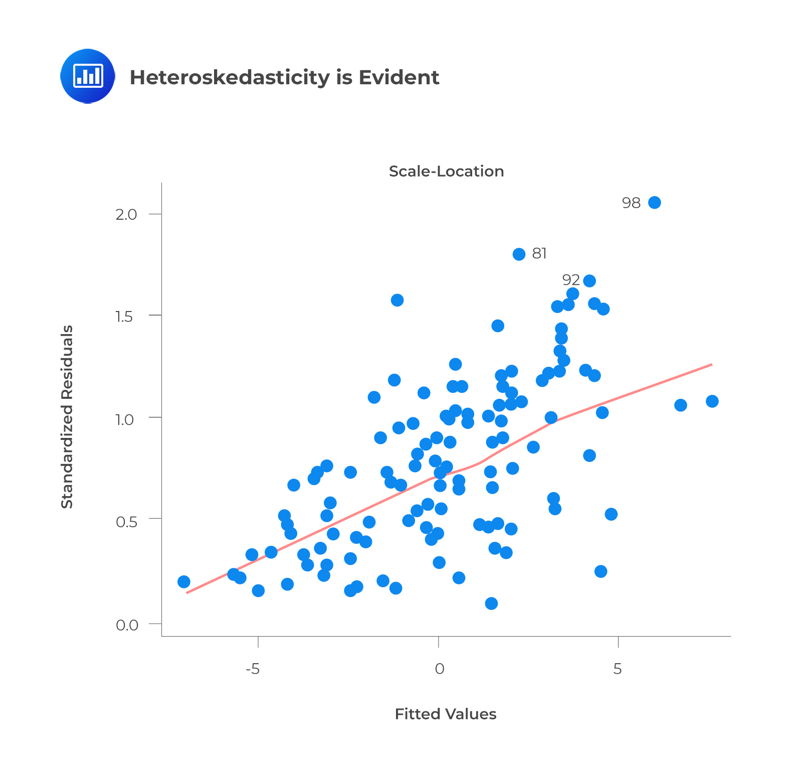
   Whenever heteroskedasticity occurs, confidence intervals for out-of-sample predictions become unrealistically large or small. If a residuals versus fitted values plot exhibits heteroskedasticity, the plot will show a funnel shape. Alternatively, you can conduct a Breusch-Pagan/Cook-Weisberg or White general test.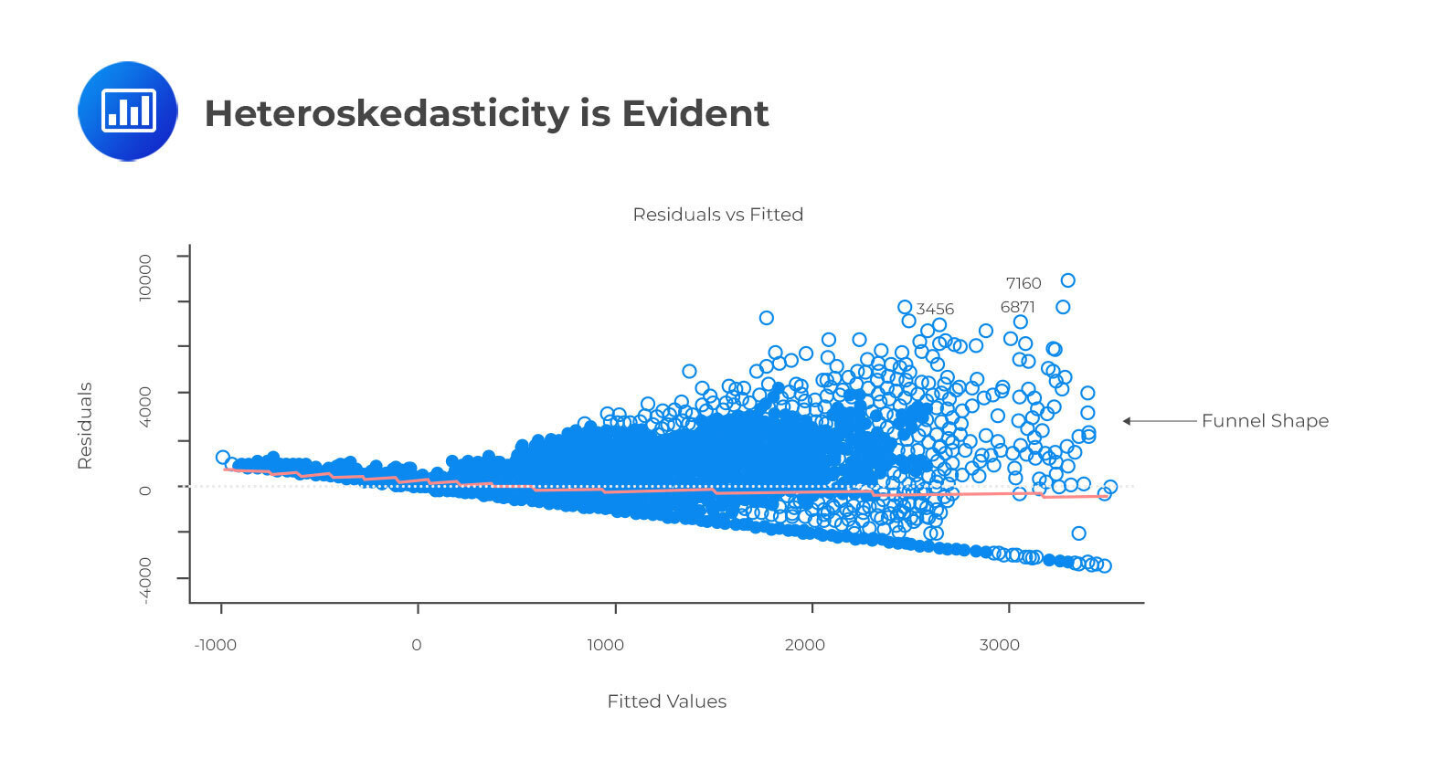

   Aside from detecting homoskedasticity, the above plot is used to determine variance equality. As you can see, the residuals are spread out along the range of predictors. It uses standardized residual values instead of residuals versus fitted values.

5. Normal Distribution of error terms: Confidence intervals may be too wide or narrow if the error terms are not normally distributed. Using least squares to minimize coefficients becomes difficult once confidence intervals become unstable. If non-normal distributions are present, there will probably be some unusual data points that will need to be closely examined to make a better model.

   The best way to determine the normal distribution of error terms is to plot a QQ plot. Kolmogorov-Smirnov and Shapiro-Wilk tests can also be used to test for normality.
   

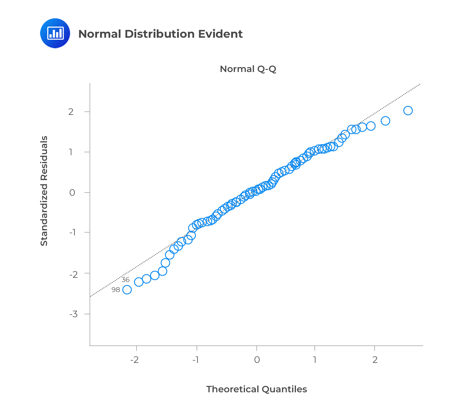
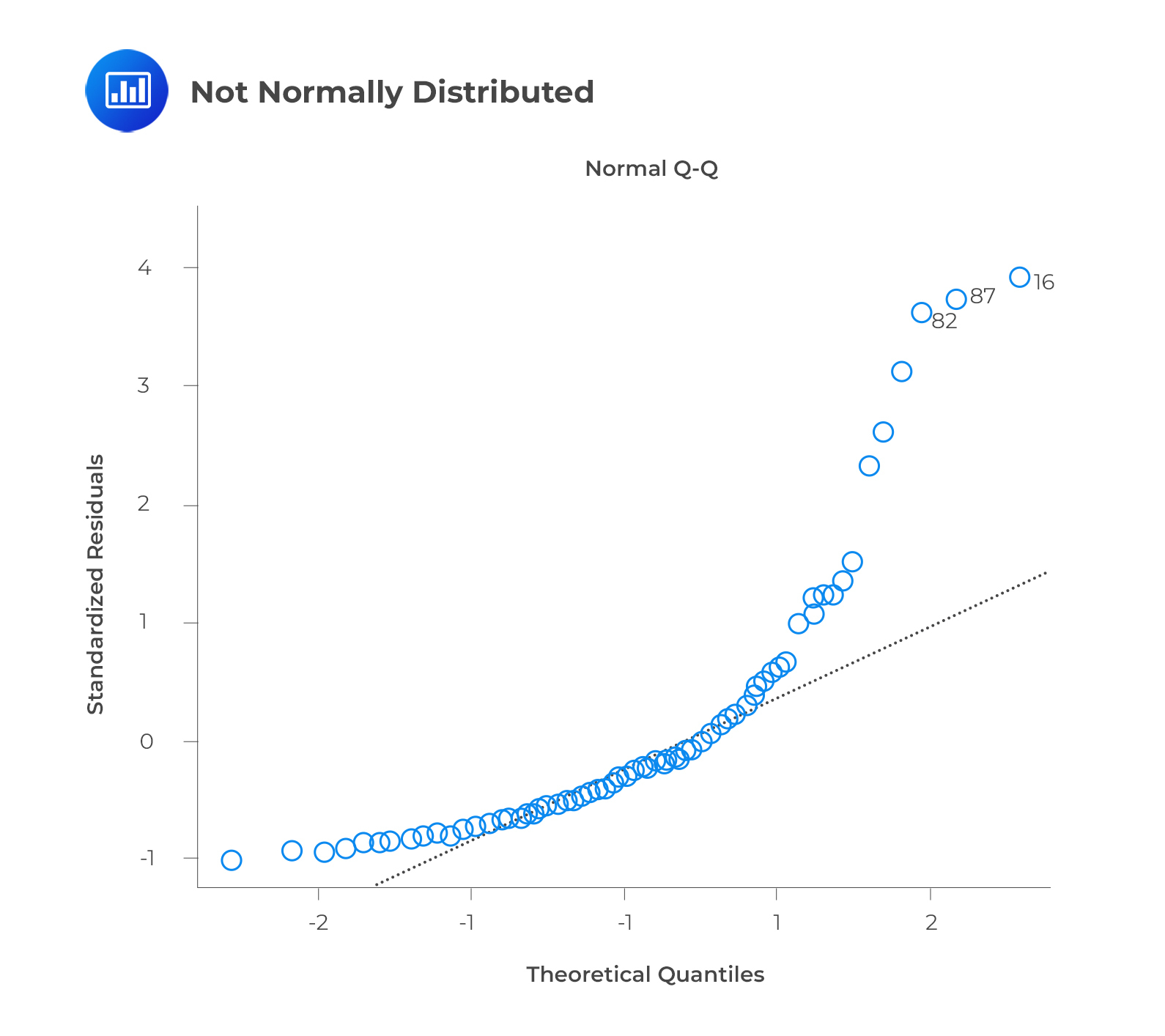
   The q-q or quantile-quantile plot is used to verify the assumption that a data set follows a normal distribution. We can determine whether the data follows a normal distribution with this plot. There would be a fairly straight line on the plot if that were the case. Note that the straight line deviates when there is no normality in the errors.

Question

Which of the following is least likely an assumption of the multiple linear regression model?

1. The independent variables are not random.
2. The error term is correlated across all observations.
3. The expected value of the error term, conditional on the independent variables, is equal to zero.

Solution

The correct answer is B.

The error term is uncorrelated across all observations.

$$ E\left(\epsilon_i\epsilon_j\right)=0\ \ \forall\ i\neq j $$

Other assumptions of the classical normal multiple linear regression model include the following:

1. The independent variables are not random. Additionally, there is no exact linear relationship between two or more independent variables.
2. The error term is normally distributed.
3. The expected value of the error term, conditional on the independent variables, is equal to 0.
4. The variance of the error term is the same for all observations.
5. A linear relation exists between the dependent variable and the independent variables.

A and C are incorrect. They both indicate the correct assumptions of the multiple linear regression model.