Role of Gamma Risk in Options Trading
Gamma measures the risk that remains once a portfolio is delta neutral (non-linearity... Read More
ANOVA is a statistical procedure used to partition the total variability of a variable into components that can be ascribed to different sources. It is used to determine the effectiveness of the independent variable(s) in explaining the variation of the dependent variable.
The F-test is performed in the analysis of variance. It tests whether the slope coefficients in a linear regression model are equal to zero. The null hypothesis for an F-test involving one independent variable is expressed as: \(H_{0}: b_{1}=0\) against the alternative hypothesis \(H_{a}: B_{1}≠0\).
The calculation of the F-statistic requires the following values:
The regression sum of squares is the measure of the explained variation in the dependent variable.
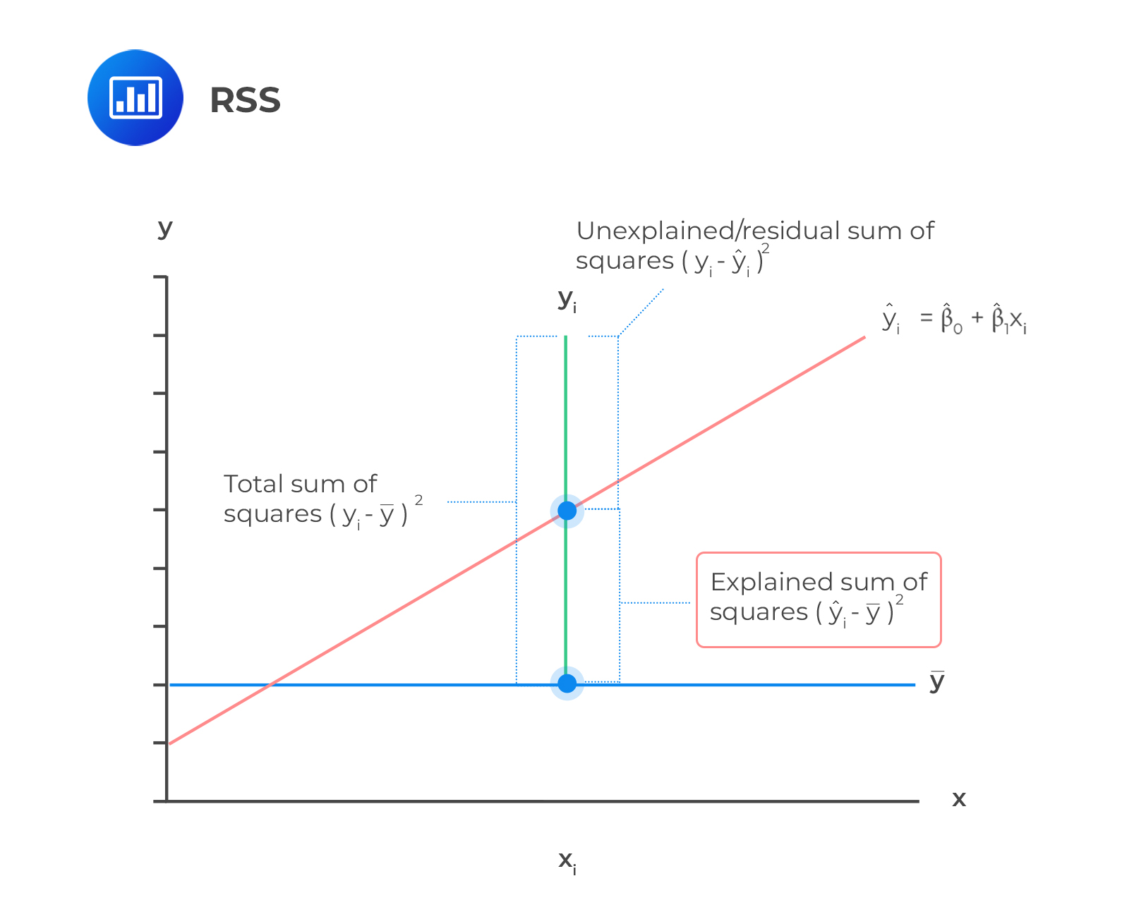 It is given by the sum of the squared differences of the predicted y-value \((\widehat{Y_{i}})\) means of y-observations \((\bar{Y})\). Mathematically,
$$\text{RSS}=\sum_{i=1}^{n}(\widehat{Y_{i}}- \bar{Y})^2$$
The sum of squared errors is also called the residual sum of squares. It is defined as the variation of the dependent variable unexplained by the independent variable.
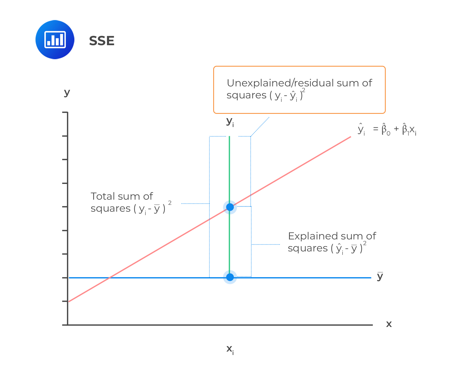 SSE is given by the sum of the squared differences of the actual y-value \((Y_{i})\) and the predicted y-values \((\widehat{Y_{i}})\). Mathematically,
$$\text{SSE}=\sum_{i=1}^{n}(Y_i-\widehat{Y_{i}})^2$$
This is a measure of the total variation of the dependent variable. The components of the total variation are shown in the following figure.
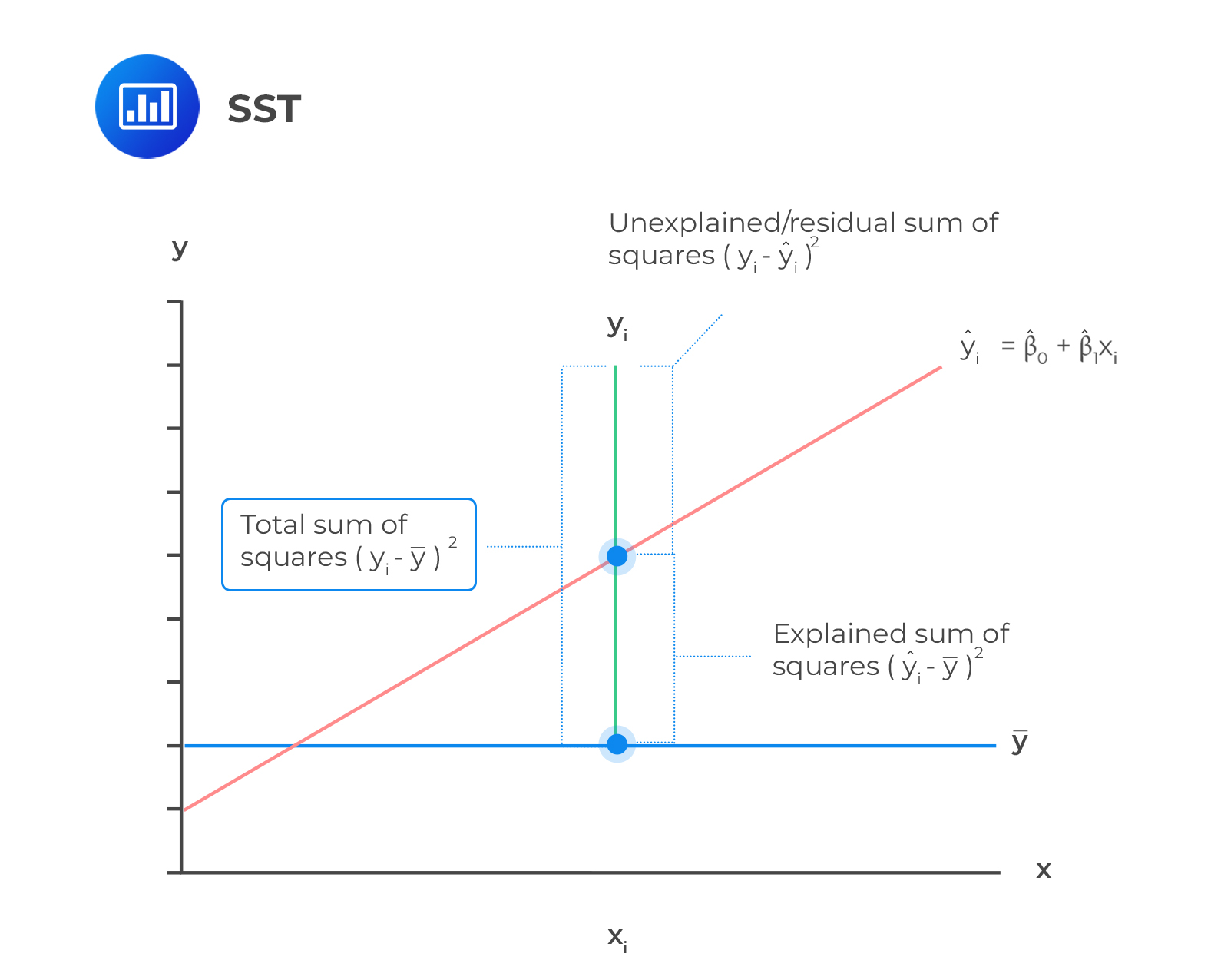 Total sum of squares is the sum of the squared differences of the actual y-value and mean of y-observations. Mathematically,
$$\text{SST}=\sum_{i=1}^{n}(Y_i-\bar{Y_{i}})^2$$
Exam tip: Total Variation = Explained Variation + Unexplained Variation, i.e., SST = SSE + RSS
The standard error of the estimate (se), also known as the root mean square error or the standard error of the regression, can be calculated from the ANOVA table. The se measures the distance between values predicted from the estimated regression and the observed values of the dependent variable. A smaller se indicates a better fit of the model. The standard error of the estimate is an absolute measure that measures how far the distance of the observed dependent variables is from the regression line. The standard error of estimate is calculated as follows.
$$S_e=\sqrt{\text{MSE}}$$
$$S_e=\sqrt\frac{{\sum_{i=1}^n({Y_i}-\hat{Y})^2}}{{n-2}}$$
Results of the ANOVA procedure are set out in an ANOVA table:
$$ {\begin{array}{l|c|c|c}\textbf{Source of Variation} & \textbf{Degrees of} & \textbf{Sum of} & \textbf{Mean Sum of}\\ & \textbf{Freedom} & \textbf{Squares} & \textbf{Squares} \\ \hline {\text{Regression (Explained)}} & 1 & \text{RSS} & \text{MSR}=\frac{\text{RSS}}{1}\\ \hline {\text{Residual (Unexplained)}} & \text{n-2} & \text{SSE} & \text{MSE}=\frac{\text{SSE}}{n-2}\\ \hline \text{Total} & \text{n-1} & \text{SST} &{}\\ \end{array}}$$
NB: The mean sum of squares (MSR) and the mean squared errors are the RSS and SSE divided by their respective degrees of freedom.
You can also use the ANOVA table results to calculate R2 and SEE using the formulas below.
$$\begin{align*}R^{2}&= \frac{\text{Total Variation (SST)}-\text{Unexpected Variation (SSE)}}{\text{Total Variation (SST)}}\\&=\frac{\text{Explained Variation (RSS)}}{\text{Total Variation (SST)}}\end{align*}$$
And,
$$\text{SEE}=\sqrt{MSE}$$
An F-test is used to determine the effectiveness of independent variables in explaining the variation of the dependent variable.
The F-test can be carried out with more than one independent variable (see more of this in the next reading on Multiple Regression). The F-statistic denoted as \(F_{1,n-2}\), for a linear regression model with one independent variable is determined as:
$$F=\frac{\text{Average Regression Sum of Squares (RSS)}}{\text{Average Sum of Squared Errors (SSE)}}$$
$$F=\frac{\frac{\text{RSS}}{\text{(k-1)}}}{\frac{\text{SSE}}{\text{(n-2)}}}=\frac{\text{Mean Regression Sum of Squares}}{\text{Mean squared error}}$$
Where:
A large F-statistic value means that the regression model does a good job in explaining the variation in the dependent variable and vice versa. Contrary, an F-statistic of 0 indicates that the independent variable does not explain variation in the dependent variable.
We reject the null hypothesis if the calculated value of the F statistic is greater than the critical F-value.
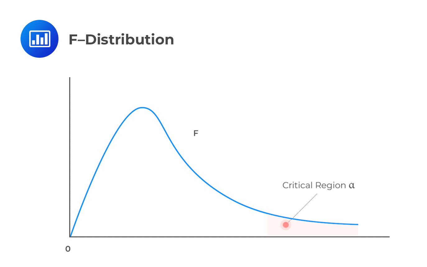 It is worth mentioning that F-statistics are not commonly used in regressions with one independent variable. This is because F-statistic is equal to the square of the t-statistic for the slope coefficient, which implies the same thing as the t-test.
The completed ANOVA table for the inflation rate and unemployment rate example is given below:
$$ {\begin{array}{c|c|c|c}\textbf{Source of} & \textbf{Degrees of} & \textbf{Sum of} & \textbf{Mean Sum of}\\ \textbf{Variation} & \textbf{Freedom} & \textbf{Squares} & \textbf{Squares} \\ \hline {\text{Regression} } & 1 & \text{RSS} = 0.004249 & \text{MSR} = 0.004249\\ \text{(Explained)} & & & \\ \hline {\text{Residual} } & 8 & \text{SSE}= 0.002686 & \text{MSE} = 0.0001492 \\ \text{(Unexplained)} & & & \\ \hline\text{Total} & 9 & \text{SST} = 0.006935 & {}\\ \end{array}}$$
a. Use the above ANOVA table to calculate the F-statistic.
b. Test the hypothesis that the slope coefficient is equal to zero at the 5% significance level.
$$\begin{align*} F & =\frac{\text{Mean Regression Sum of Squares (MRS)}}{\text{Mean Squared Error (MSE)}} \\ F&=\frac{004249}{0.0001492}\\&=28.48\end{align*}$$
We are testing the null hypothesis \(H_0:b_{1}=0\) against the alternative hypothesis \(H_1:b_1≠0\). The critical F-value for \(k=1\) and \(n-2=8\) degrees of freedom at a 5% significance level is roughly 5.32. Note that this is a one-tail test; therefore, we use the 5% F-table.
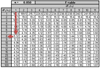
Recall that the null hypothesis is rejected if the calculated value of the F-statistic is greater than the critical value of F. Since \(28.48>5.32\), we reject the null hypothesis and conclude that the slope coefficient is significantly different from zero. Notice that we also rejected the null hypothesis in the previous examples as the 95% confidence interval did not include zero.
F-test duplicates the t-test for the slope coefficient significance for a linear regression model with one independent variable. In this case, \(t^{2}=2.306^2≈5.32\). Since F-statistic is the square of the t-statistic for the slope coefficient, it infers the same thing as the t-test. However, this is not the case for multiple regressions.
Exam tip: Concentrate on the application of the F-test under a multiple regression framework.
Question
Consider the following analysis of variance (ANOVA) table:
$$\small{\begin{array}{c|c|c|c} \textbf{Source of Variation} & \textbf{Degrees of} & \textbf{Sum of} & \textbf{Mean Sum of}\\ & \textbf{Freedom} & \textbf{Squares} & \textbf{Squares} \\ \hline \text{Regression (Explained)} & 1 & \text{RSS} = 1,701,563 & \text{MSR} = 1,701,563\\ \hline\text{Residual (Unexplained)} & 3 & \text{SSE}= 106,800 & \text{MSE} = 13,350\\ \hline\text{Total} & 4 & \text{SST} = 1,808,363 &{} \\ \end{array}}$$
The value of \(R^{2}\) and F-statistic for the test of fit of the regression model are closest to:
- 6% and 16, respectively.
- 94% and 127, respectively.
- 99% and 127, respectively.
Solution
The correct answer is B.
$$\begin{align*}R^{2}&= \frac{\text{Explained Variation (RSS)}}{\text{Total Variation}}\\&=\frac{1,701,563}{1,808,363}\\&=0.94\\&=94\%\end{align*}$$
$$\begin{align*} F & =\frac{\text{Mean Regression Sum of Squares (MSR)}}{\text{Mean Squared Error (MSE)}} \\ F&=\frac{1,701,563}{13,350}\\&=127.46 \approx 127\end{align*}$$
Reading 0: Introduction to Linear Regression
LOS 0 (e) Describe the use of analysis of variance (ANOVA) in regression analysis, interpret ANOVA results, and calculate and interpret the standard error of estimate in a simple linear regression
Get Ahead on Your Study Prep This Cyber Monday! Save 35% on all CFA® and FRM® Unlimited Packages. Use code CYBERMONDAY at checkout. Offer ends Dec 1st.