


Binomial Interest Rate Model
Modeled future interest rates can take on different possible values, depending on the... Read More

A hedging portfolio can be created by going long \(\phi\) units of the underlying asset and going short the call option such that the portfolio has an initial value of:
$$ V_0=\phi S_0-c_0 $$
Where:
\(S_0\) = The current stock price
\(c_0\) = Current call value
After a one-time-period, this portfolio will be worth:
\(V_1 =\phi S_ou-c_u\) if the asset price jumps up
or
\(V_1 =\phi S_od-c_d\) if the asset price jumps down
If we equate the values of the up and down portfolios, the number of units of the underlying asset can be obtained as:
$$ \phi=\frac{c_u-c_d}{S_0u-S_0d} $$
\({\phi}\) is referred to as the hedge ratio. It is the ratio that makes a trader indifferent to the movement of the underlying asset price. An arbitrageur creates a hedged portfolio to eliminate price risk. This way, they satisfy Rule 2: “Do not take any price risk.”
Suppose at time step 0, a trader borrows the present value of:
$$ -\phi S_od+c_d $$
Assuming there is no-arbitrage, we shall have:
$$ c_0-\phi S_0 = PV(–\phi S_0d + c_d ) $$
Since \(–\phi S_0d + c_d= –\phi S_0u+ c_u\).
This is can also be expressed as:
$$ c_0–\phi S_0 = PV– \phi S_0u + c_u $$
The no-arbitrage single-period valuation approach leads to the following single-step call option valuation equation for call options:
$$ \begin{align*} c_0 &=\phi S_0 + PV(–\phi S_0d + c_d) \\ c_0 & =\phi S_0 + PV(–\phi S_0u + c_u) \end{align*} $$
Therefore, a call option is similar to owning \(\phi\) units of the underlying asset and borrowing \(PV(-\phi S_od+c_d)\). This makes the transaction completely arbitrage-free, hence satisfying Rule 1: “Do not use own money.” Moreover, we can view a call option as a leveraged position in the underlying asset.
We can use the idea that a hedged portfolio returns the risk-free rate to determine the initial value of a call or a put option.
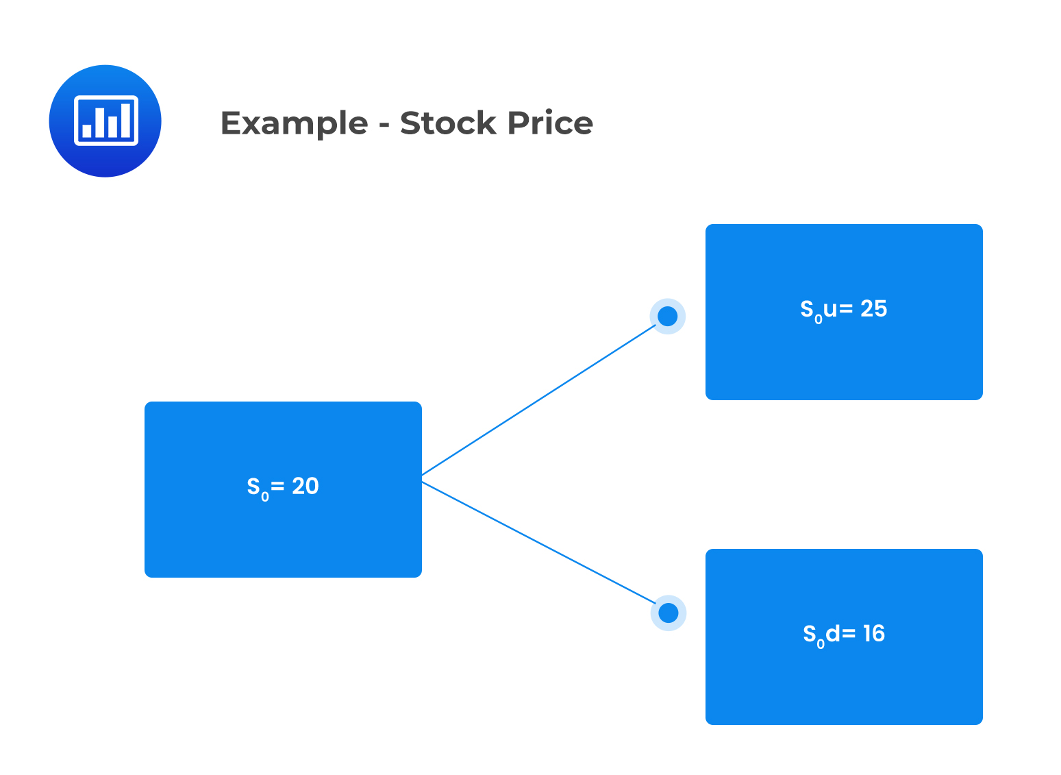
Consider a one-period binomial model of a non-dividend-paying stock whose current price is $20. Assume that:
The current value of a one-period European call option that has an exercise price of $20 is closest to:
The binomial tree in respect of the stock price is as follows:
 Similarly, consider a corresponding binomial tree with respect to the payoff provided by the call option at time 1, i.e., the profit paid at exercise:
 We can determine \(c_0\) by using the single-period call option valuation equation as follows:
$$ \begin{align*} c_0 &=\phi S_0 + PV(– \phi S_d + c_d) \\ \phi &=\frac{c_u-c_d}{S_0u-S_0d} \\ \phi &=\frac{5-0}{25-16}=0.56 \end{align*} $$
Therefore,
$$ c_0=0.56\times20+e^{-0.04}\left[-0.56\times16+0\right]=$2.59 $$
This implies that buying a call option for $2.59 is equivalent to buying 0.56 units of the underlying stock for $11.20 and lending $8.61 such that the effective payment is $2.59.
The no-arbitrage single period valuation equation for put options is expressed as:
$$ p=\phi S_0+PV\left(-\phi S_0d+p_d\right) $$
Equivalently,
$$ p=\phi S_0+PV\left(-\phi S_0u+p_u\right) $$
Where the hedge ratio, \(\phi\), is given as:
$$ \phi=\frac{p_u-p_d}{S_0u-S_0d} \le 0 $$
Note that the hedge ratio, in this case, will be negative as \(p_u\) is less than \(p_d\). Therefore, the arbitrageur should short-sell the underlying and lend a portion of the proceeds to replicate a long-put position.
Therefore, a put option can be viewed as equivalent to shorting the underlying asset and lending \(PV– \phi S_0 u + p_u\).
Consider a one-period binomial model of a non-dividend-paying stock whose current price is $20. Assume that:
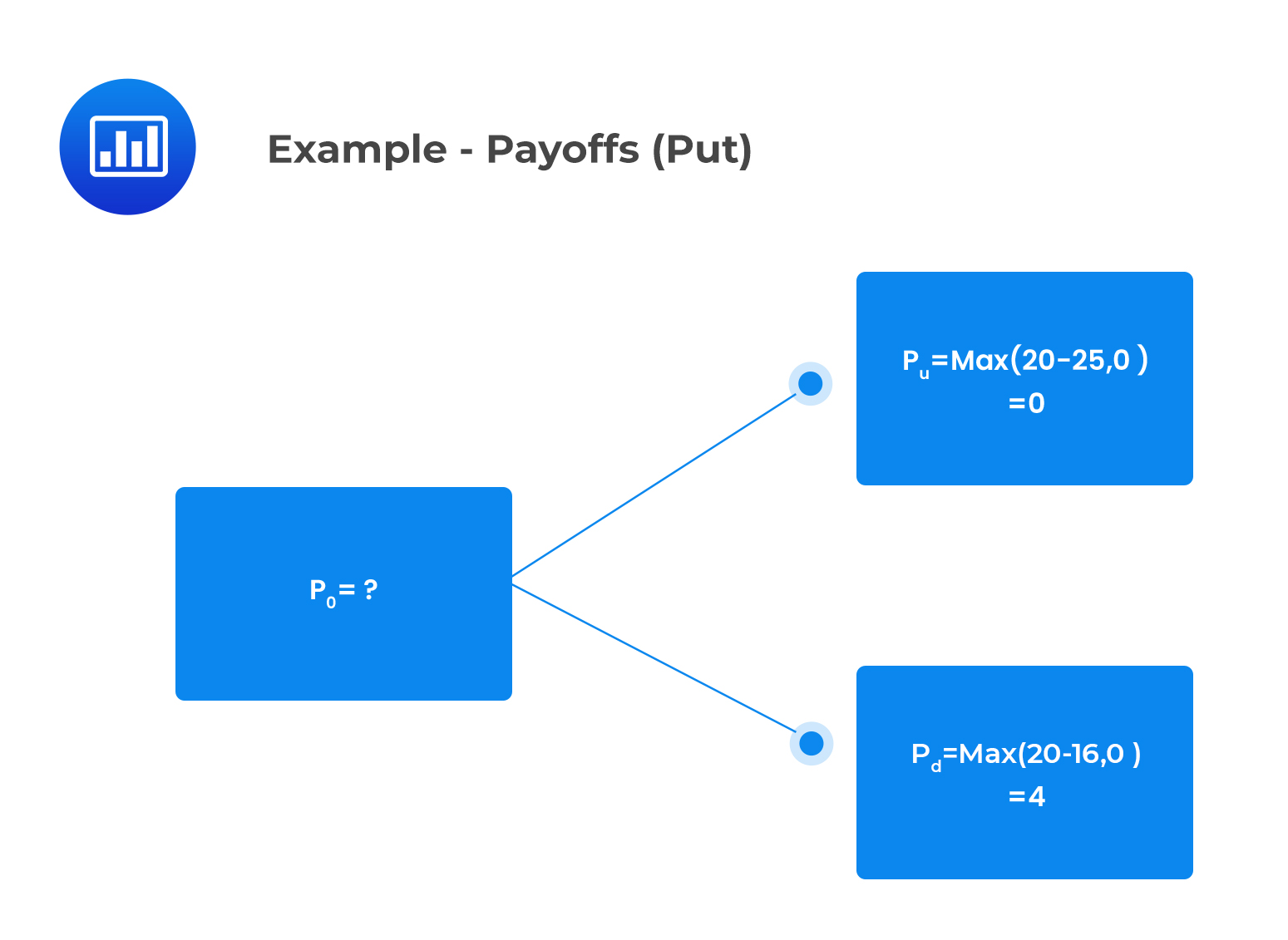
The current value of a one-period European put option that has an exercise price of $20 is closest to:
The payoff provided by the put option at time one is represented in the following binomial tree:
 $$ p=\phi S_0+PV– \phi S_0 u + p_u $$
Where:
$$ \begin{align*} \phi &=\frac{p_u-p_d}{S_0u-S_0d}\le0 \\ \phi &=\frac{0-4}{25-16}=-0.44 \\ p & =-0.44\times20+e^{-0.04}\left(–0.44\times25+0\right)=$1.77 \end{align*} $$
Notice that buying a put option for $1.77 is equivalent to short selling 0.44 units of the underlying stock for $8.80 and lending $10.57.
Consider a one-period binomial model of a non-dividend-paying stock whose current price is $20. Imagine that:
In the previous section, we determined the current value of this call option as $2.59, given a strike price of $20.
Now, assume that the call option has a market price of $4.50. Assuming that we trade 1,000 call options, we can illustrate how this opportunity can be exploited to earn an arbitrage profit.
Since the call option is overpriced, we will sell 1,000 call options and buy several shares of the underlying determined by the hedge ratio.
$$ \begin{align*} \phi & =\frac{c_u-c_d}{S_0u-S_0d} \\ \phi &=\frac{$5-$0}{$25-$16}=\frac{5}{9} \text{ shares per option} \end{align*} $$
Therefore, we will purchase \(1,000\times\frac{5}{9}=555.5555 \text{ shares}\).
The net cost of a portfolio with 555.55 shares of the stock held long at $20 per share and 1,000 calls held short at $4.50 is:
$$ \text{Net cost of the portfolio}=\left(555.55\times$20\right)-\left(1,000\times$4.50\right)\approx$6,611 $$
The portfolio value will be the same at maturity regardless of whether the stock price moves up to $25 or down to $16.
The value of the portfolio after stock price moves up is:
$$ V_u = \left(555.55 \times $25\right) – 1,000 \times $5 \approx $8,889 $$
The value of the portfolio after stock price moves down is:
$$ V_d= \left(555.55 \times $16\right)– 1,000 × $0\approx $8,889 $$
The arbitrage profit on this portfolio at the end of one year if the price moves up or down after repayment of the loan is $8,889 – $6,875 = $2,014.
The discounted value of the arbitrage profit is therefore:
$$ PV \left(\text{Arbitrage profit} \right)=\frac{$2,014}{1.04}=$1,936.54 $$
Question
Consider a non-dividend-paying stock with a current price of $50 and an exercise price of $50. The stock price can be modeled by assuming that it will either increase by 12% or decrease by 10% each year, independent of the price movement in other years. A trader constructs a portfolio consisting of 100 call options. If a call option is overpriced, which portfolio most likely leads to an arbitrage profit?
- Buy 100 call options, short 54.55 shares.
- Buy 100 call options, short 45.45 shares.
- Sell 100 call options, buy 54.55 shares.
Solution
The correct answer is C.
\(u=1.12\)
\(d=0.90\)
We can represent the above information in the following binomial tree:
The call payoffs are as follows:
$$ \begin{align*} c_u &=max{\left($56-$50,0\right)}=$6 \\ c_d &=max{\left($45-50,0\right)}=$0 \end{align*} $$
Since the option is overpriced, the trader will sell 100 call options and purchase several shares determined by the hedge ratio:
$$ \begin{align*} \phi &=\frac{c_u-c_d}{S_0u-S_0d} \\ \phi &=\frac{$6-$0}{$56-$45}=0.5455 \text{ shares per option} \end{align*} $$
$$ \text{Total number of shares to purchase} = 100 \times 0.5455 = 54.55 $$
Buying 54.55 shares of stock will produce a riskless hedge. The payoff at expiry will return more than the risk-free rate on the hedge portfolio’s net cost. Borrowing to finance the hedge portfolio and earning a higher rate than the borrowing rate produces riskless profits.
Reading 34: Valuation of Contingent Claims
LOS 34 (c) Identify an arbitrage opportunity involving options and describe the related arbitrage.
Review how to identify arbitrage opportunities involving options and describe the related arbitrage with CFA Level 2 study notes, practice questions, mock exams, and video lessons designed to strengthen your exam preparation.
Offered by AnalystPrep


Get Ahead on Your Study Prep This Cyber Monday! Save 35% on all CFA® and FRM® Unlimited Packages. Use code CYBERMONDAY at checkout. Offer ends Dec 1st.