


Determine conditional and marginal pro ...
Marginal Probability Distribution In the previous reading, we looked at joint discrete distribution... Read More

In the previous reading, we looked at joint discrete distribution functions. In this reading, we will determine conditional and marginal probability functions from joint discrete probability functions.
Suppose that we know the joint probability distribution of two discrete random variables, \(X\) and \(Y\), and that we wish to obtain the individual probability mass function for \(X\) or \(Y\). These individual mass functions of \(X\) and \(Y\) are referred to as the marginal probability distribution of \(X\) and \(Y\), respectively.
Once we have these marginal distributions, we can analyze the two variables separately.
Recall that the joint probability mass function of the discrete random variables \(X\) and \(Y\), denoted as \(f_{XY}(x,y)\), satisfies the following properties:
Let \(X\) and \(Y\) have the joint probability mass function \(f(x,y)\) defined on the space \(S\).
The probability mass function of \(X\) alone, which is called the marginal probability mass function of X, is given by:
$$ f_x\left(x\right)=\sum_{y}{f\left(x,y\right)=P\left(X=x\right),\ \ \ \ \ x\epsilon S_x} $$
Where the summation is taken over all possible values of \(y\) for each given \(x\) in space \(S_X\).
Similarly, the marginal probability mass function of Y is given by:
$$ f_y\left(y\right)=\sum_{x}{f\left(x,y\right)=P\left(Y=y\right),\ \ \ \ \ \ y\epsilon S_y} $$
where the summation is taken over all possible values of \(x\) for each given \(y\) in space \(S_y\).
The data for an insurance company’s policyholders is characterized as follows:
$$ \begin{array}{c|ccc|c}
\bf{R} & \bf{X} & & & \\
\textbf{Risk Class} & \textbf{Loss} & \textbf{Amount} & & \\
& 0 & 50 & 100 & \textbf{Totals} \\ \hline
{0 (\text{Low}) } & 0.18 & 0.09 & 0.03 & 0.30 \\ \hline
{1 (\text{Medium})} & 0.12 & 0.30 & 0.18 & 0.60 \\ \hline
{2 (\text{High})} & 0.02 & 0.03 & 0.05 & 0.10 \\ \hline
\textbf{Total} & 0.32 & 0.42 & 0.26 & 1.00
\end{array} $$
Given the joint probability distribution above, we may be interested to know what are the probabilities of, say: i) a low-risk individual; ii) a medium-risk individual; iii) a high-risk individual; or the probability of getting: i) a loss amount of 0; ii) a loss amount of 50; iii) a loss amount of 100.
To find the marginal probability of \(R\), i.e., the probability of a low-risk individual, a medium-risk individual, or a high-risk individual, we will add across each column, i.e.,
$$ P\left(R=0\right)=P\left(R=0\cap X=0\right)+P\left(R=0\cap X=50\right)+P\left(R=0\cap X=100\right) $$
$$ f_R\left(0\right)=0.18+0.09+0.03=0.30 $$
Similarly,
$$ P\left(R=1\right)=f_R\left(1\right)=0.12+0.30+0.18=0.60 $$
And
$$ P\left(R=2\right)=f_R\left(2\right)=0.02+0.03+0.05=0.10 $$
We can do the same to find probabilities of getting different loss amounts, i.e., the marginal probability of \(X\):
$$ P\left(X=0\right)=P\left(R=0\cap X=0\right)+P\left(R=1\cap X=0\right)+P\left(R=2\cap X=0\right) $$
$$ {\Rightarrow f}_X\left(0\right)=0.18+0.12+0.02=0.32 $$
Similarly,
$$ P\left(X=50\right)=f_X\left(50\right)=0.09+0.03+0.05=0.42 $$
And,
$$ P\left(X=100\right)=f_X\left(100\right)=0.03+0.18+0.05=0.26 $$
The marginal distributions of \(R\) and \(X\) are as follows:
$$ \begin{array}{c|c}
R & Pr=f_R(r) \\ \hline
0 & 0.30 \\ \hline
1 & 0.60 \\ \hline
2 & 0.10
\end{array} \\
\begin{array}{c|c}
X & Pr=f_R(r) \\ \hline
0 & 0.32 \\ \hline
50 & 0.42 \\ \hline
100 & 0.26
\end{array} $$
Suppose that the joint p.m.f of \(X\) and \(Y\) is given as:
$$ f\left(x,y\right)=\frac{x+y}{21},\ \ \ x=1, 2\ \ \ y=1, 2, 3 $$
Solution
$$ f_x\left(x\right)=\sum_{y}{f\left(x,y\right)=P\left(X=x\right),\ \ \ x\epsilon S_x} $$
Thus,
$$ \begin{align*}
f_x\left(x\right) & =\sum_{y=1}^{3}{\frac{x+y}{21} } \\
& =\frac{x+1}{21}+\frac{x+2}{21}+\frac{x+3}{21}=\frac{3x+6}{21}, \ \ \ \text{ for } x=1,2
\end{align*} $$
$$ f_y\left(y\right)=\sum_{x}{f\left(x,y\right)=P\left(Y=y\right),\ \ \ \ y\epsilon S_y} $$
Thus,
$$ \begin{align*}
f_Y\left(y\right) & =\sum_{x=1}^{2}{\frac{x+y}{21}} \\
& = \frac{1+y}{21}+\frac{2+y}{21}=\frac{3+2y}{21},\ \ \ \text{for } y=1, 2, 3
\end{align*} $$
\(X\) and \(Y\) have the joint probability function as given in the table below:
$$ \begin{array}{c|c|c|c} {\quad \text X }& {1} & {2} & {3} \\ {\Huge \diagdown } & & & \\ {\text Y \quad} & & & \\ \hline
{1} & 0.12 & 0.15 & 0 \\ \hline {2} & 0.13 & 0.05 & 0.03 \\ \hline {3} & {0.18} & {0.06} & {0.07} \\ \hline 4 & 0.17 & 0.04 & \\ \end{array} $$
Determine the probability distribution of \(X\).
Solution
We know that:
$$ f_x\left(x\right)=\sum_{y}{f\left(x,y\right)=P\left(X=x\right),\ \ \ \ \ x\epsilon S_x} $$
So that the marginal probabilities are:
$$ \begin{align*}
P\left(X=1\right) & =0.12+0.13+0.18+0.17=0.6 \\
P\left(X=2\right) & =0.15+0.05+0.06+0.04=0.3 \\
P\left(X=3\right) & =0.03+0.07=0.1
\end{align*} $$
Therefore, the marginal probability distribution of \(X\) is:
$$ \begin{array}{c|c|c|c}
X & 1 & 2 & 3 \\ \hline
P(X=x) & 0.6 & 0.3 & 0.1
\end{array} $$
Conditional probability is a key part of Baye’s theorem. In plain language, it is the probability of one thing being true, given that another thing is true. It differs from joint probability, which is the probability that both things are true without knowing that one of them must be true. For instance:
We can use a Euler diagram to illustrate the difference between conditional and joint probabilities. Note that, in the diagram, each large square has an area of 1.
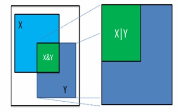
Let \(X\) be the probability that a patient’s left kidney is infected, and let \(Y\) be the probability that the right kidney is infected. The green area on the left side of the diagram represents the probability that both of the patient’s kidneys are affected. This is the joint probability \((X, Y)\). If \(Y\) is true (e.g., given that the right kidney is infected), then the space of everything, not \(Y\), is dropped, and everything in \(Y\) is rescaled to the size of the original space. The rescaled green area on the right-hand side is now the conditional probability of \(X\) given \(Y\), expressed as \(P(X|Y)\). Put differently, this is the probability that the left kidney is infected if we know that the right kidney is affected.
It is worth noting that the conditional probability of \(X\) given \(Y\) is not necessarily equal to the conditional probability of \(Y\) given \(X\).
Recall that for the univariate case, the conditional distribution of an event \(A\) given \(B\) is defined by:
$$ P\left(A\middle|B\right)=\frac{P\left(A\cap B\right)}{P\left(B\right)},\ \ \ \text{provided that } P\left(B\right) \gt 0$$
Where event \(B\) happened first and impacted how \(A\) occurred. We can extend this idea to multivariate distributions.
Let \(X\) and \(Y\) be discrete random variables with joint probability mass function, \(f(x, y)\) defined on the space \(S\).
Also, let \(f_x\left(x\right)\) and \(f_y\left(y\right)\) be the marginal distribution function of \(X\) and \(Y\), respectively.
The conditional probability mass function of X, given that \({Y}={y}\), is given by:
$$ g\left(x\middle|y\right)=\frac{f\left(x,y\right)}{f_Y\left(y\right)},\ \ \ \text{provided that } f_Y\left(y\right) \gt 0 $$
Similarly, the conditional probability mass function of Y, given that \({X}={x}\), is defined by;
$$ h\left(y\middle|x\right)=\frac{f\left(x,y\right)}{f_X\left(x\right)},\ \ \ \text{provided that } f_X\left(x\right) \gt 0, $$
The data for an insurance company’s policyholders is characterized as follows:
$$ \begin{array}{c|ccc}
\bf R & \bf{X} & & \\
\textbf{Risk Class} & \textbf{Loss} & \textbf{Amount} & \\ \hline
& 0 & 50 & 100 \\ \hline
0 (\text{Low}) & 0.18 & 0.09 & 0.03 \\ \hline
1 (\text{Medium}) & 0.12 & 0.30 & 0.18 \\ \hline
2 (\text{High}) & 0.02 & 0.03 & 0.05
\end{array} $$
We can find the conditional probabilities for \(X|R=0\):
$$ \begin{align*}
P\left(X=0\right|R=0) &=\frac{P(R=0\cap X=0)}{P(R=0)}=\frac{0.18}{0.30}=0.6 \\
P\left(X=50\right|R=0) & =\frac{P(R=0\cap X=50)}{P(R=0)}=\frac{0.09}{0.30}=0.30 \\
P\left(X=100\right|R=0) &=\frac{P(R=0\cap X=100)}{P(R=0)}=\frac{0.03}{0.30}=0.10
\end{align*} $$
Note that,
$$ \text{Conditional probability}=\frac{\text{Joint probability}}{\text{Marginal probability}} $$
Now, the conditional distribution of \(X|R=0\) is:
$$ \begin{array}{c|c}
X|R=0 & P=f_{X|R=0}(x) \\ \hline
0 & 0.60 \\ \hline
50 & 0.30 \\ \hline
100 & 0.10
\end{array} $$
Let \(X\) be the number of days of sickness over the last year, and let \(Y\) be the number of days of sickness this year. \(X\) and \(Y\) are jointed distributed as in the table below:
$$ \begin{array}{c|c|c|c} {\quad \text X }& {0} & {1} & {2} \\ {\Huge \diagdown } & & & \\ {\text Y \quad} & & & \\ \hline {1} & {0.1} & {0.1} & {0} \\ \hline {2} & {0.1} & {0.1} & {0.2} \\ \hline {3} & {0.2} & {0.1} & {0.1} \end{array} $$
Determine:
Solution
$$ P\left(X=x\right)=\sum_{y}{P\left(x,y\right)\ \ \ \ \ x\epsilon S_x} $$
Therefore, we have:
$$ \begin{align*} P\left(X=0\right) & =0.1+0.1+0.2=0.4 \\ P\left(X=1\right) &=0.1+0.1+0.1=0.3 \\ P\left(X=2\right)& =0+0.2+0.1=0.3 \end{align*} $$
When represented in a table, the marginal distribution of \(X\) is:
$$ \begin{array}{c|c|c|c}
X & 0 & 1 & 2 \\ \hline
P(X=x) & 0.4 & 0.3 & 0.3
\end{array} $$
$$ P\left(Y=y\right)=\sum_{x}{P\left(x,y\right),\ \ \ \ y\epsilon S_y} $$
Therefore, we have:
$$ \begin{align*} P\left(Y=1\right) &=0.1+0.1+0=0.2 \\ P\left(Y=2\right) & =0.1+0.1+0.2=0.4 \\ P\left(Y=3\right)&=0.2+0.1+0.1=0.4 \end{align*} $$
Therefore, the marginal distribution of \(Y\) is:
$$ \begin{array}{c|c|c|c}
Y & 1 & 2 & 3 \\ \hline
P(Y=y) & 0.2 & 0.4 & 0.4
\end{array} $$
$$ \begin{align*}
P\left(Y=1\middle|X=2\right) & =\frac{P\left(Y=1, X=2\right)}{P\left(X=2\right)}=\frac{0}{0.3}=0 \\
P\left(Y=2\middle|X=2\right) & =\frac{P\left(Y=2, X=2\right)}{P\left(X=2\right)}=\frac{0.2}{0.3}=0.67 \\
P\left(Y=3\middle|X=2\right) & =\frac{P\left(Y=3, X=2\right)}{P\left(X=2\right)}=\frac{0.1}{0.3}=0.33
\end{align*} $$
The conditional distribution is, therefore,
$$ p\left(y\middle|x=2\right)= \left\{ \begin{matrix} 0, & y =1 \\ 0.67 & y=2 \\ 0.33, & y=3 \end{matrix} \right. $$
An actuary determines that the number of monthly accidents in two towns, \(M\) and \(N\), is jointly distributed as
$$ f\left(x,y\right)=\frac{5x+3y}{81},\ \ \ \ x=1, 2,\ \ \ y=1, 2, 3. $$
Let \(X\) and \(Y\) be the number of monthly accidents in towns \(M\) and \(N\), respectively.
Find
Solution
$$ h\left(y\middle|x\right)=\frac{f\left(x,y\right)}{f_X\left(x\right)} $$
The marginal pmf of \(X\) is
$$ \begin{align*} f_X\left(x\right) & =\sum_{y}{f\left(x,y\right)=P\left(X=x\right),\ \ \ \ \ x\epsilon S_x} \\
& =\sum_{y=1}^3\frac{(5x+3y)}{81} \\
& =\frac{5x+3\left(1\right)}{81}+\frac{5x+3\left(2\right)}{81}+\frac{5x+3\left(3\right)}{81}= \frac{15x+18}{81} \\
\therefore f_X\left(x\right) & =\frac{15x+18}{81},\ \ x=1, 2
\end{align*} $$
Thus,
$$ h\left(y\middle|x\right)=\frac{\frac{5x+3y}{81}}{\frac{15x+18}{81}}=\frac{5x+3y}{15x+18},\ \ \ \ \ y=1, 2, 3,\ \text{ when } x=1 \text{ or } 2 $$
$$\begin{align*}
f_Y\left(y\right) & =\sum_{x}{f\left(x,y\right)=P\left(Y=y\right),\ \ \ \ y\epsilon S_y} \\
& =\sum_{x=1}^{2}\frac{5x+3y}{81}\\ & =\frac{5\left(1\right)+3y}{81}+\frac{5\left(2\right)+3y}{81} \\
\therefore f_Y\left(y\right) & =\frac{15+6y}{81}\ \ y=1, 2, 3. \end{align*} $$
Now,
$$ \begin{align*} g\left(x\middle|y\right) & =\frac{f\left(x,y\right)}{f_Y\left(y\right)} \\
& =\frac{\frac{5x+3y}{81}}{\frac{15+6y}{81}}=\frac{5x+3y}{15+6y} \\
\therefore g\left(x\middle|y\right)&=\frac{5x+3y}{15+6y}\ \ \ \ x=1, 2 \text{ when } y=1 \text{ or } 2 \text{ or } 3
\end{align*} $$
We can use conditional distributions to find conditional probabilities.
For example,
$$ P\left(Y=1\middle|X=2\right)=h\left(1\middle|2\right)=h\left(y\middle|x\right)=\frac{5\times 2+3\times 1}{15\times 2+18}=\frac{13}{48} $$
If we find all the probabilities for this conditional probability function, we would see that they behave similarly to the joint probability mass functions seen in the previous reading.
Now, let’s keep \({X}={2}\) fixed and check this:
$$ P\left(Y=2\middle|X=2\right)=h\left(2\middle|2\right)=\frac{5\times 2+3\times 2}{15\times 2+18}=\frac{16}{48} $$
and,
$$ P\left(Y=3\middle|X=2\right)=h\left(3\middle|2\right)=\frac{5\times 2+3\times 3}{15\times 2+18}=\frac{19}{48} $$
Summing up the above probabilities, we get
$$ P\left(Y\middle|X=2\right)=h\left(1\middle|2\right)+h\left(2\middle|2\right)+h\left(3\middle|2\right)=\frac{13}{48}+\frac{16}{48}+\frac{19}{48}=1 $$
Note that the same occurs for the conditional distribution of \(X\) given \(Y\), \({g}({x}|{y})\).
Thus, \({h}({y}|{x})\) and \({g}({x}|{y})\) both satisfy the conditions of a probability mass function, and we can do the same operations we did on joint discrete probability functions.
Question
Let’s consider an example where we are analyzing the performance of a customer support team based on the number of resolved queries (X) and the number of follow-up queries needed (Y). The joint probability mass function of \(X\) and \(Y\) is given as:
$$ f_X\left(x\right)\left(x,y\right)=\frac{x+2y}{30} $$
for x = 1, 2, 3, and y = 1, 2
Determine the marginal probability mass function of \(X\).
- \(\frac{1+x}{5}\)
- \( \frac{x+4}{30}\)
- \( \frac{x+2}{30}\)
- \( \frac{x+3}{15}\)
- \(\frac{x+3}{30} \)
Solution
The correct answer is D.
The marginal probability mass function of \(X\) is found by summing the joint probability mass function over all values of \(Y\):
$$ f_X\left(x\right)=\sum_{y}{f_{XY}\left(x,y\right)} $$
Thus,
$$ \begin{align*}
f_X\left(x\right) & =f_{XY}\left(x,1\right)+f_{XY}\left(x,2\right) \\
f_X\left(x\right) & =\frac{x+2\left(1\right)}{30}+\frac{x+2\left(2\right)}{30}=\frac{2x+6}{30}=\frac{x+3}{15}
\end{align*} $$for \(x = 1, 2\)
Learning Outcome
Topic 3. b: Multivariate Random Variables – Determine conditional and marginal probability functions for discrete random variables only.
Offered by AnalystPrep


Get Ahead on Your Study Prep This Cyber Monday! Save 35% on all CFA® and FRM® Unlimited Packages. Use code CYBERMONDAY at checkout. Offer ends Dec 1st.