Apply Transformations
Transformations allow us to find the distribution of a function of random variables.... Read More
In the previous reading, we covered the fundamental ideas of deductibles, coinsurance, benefit limits, and inflation in the context of insurance. In this reading, we will focus on more quantitative aspects. Specifically, we will perform calculations to determine the expected value, variance, and standard deviation for both the loss random variable and the corresponding payment random variable upon the application of policy adjustments.
In this reading, we will use three key random variables in our discussion. We can let:
To understand how the above random variables work, let us have a look at a number of examples:
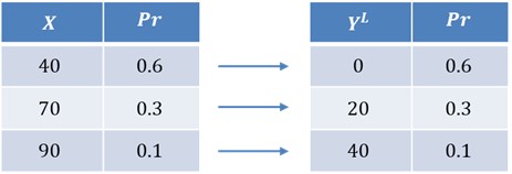
An insurance policy has a ground-up loss, \(X\), given in the table below, and a deductible of \(d=50\).
$$ \begin{array}{c|c}
X & Pr \\ \hline
40 & 0.6 \\ \hline
70 & 0.3 \\ \hline
90 & 0.1
\end{array} $$
Note that ground-up loss refers to the total amount of losses incurred from an insurance claim before any deductibles are applied.
If we let \(Y^L\) be the random variable for the insurance payment per loss, with a deductible of \(d=50\), we can create a second table such that:

A deductible means that the person being insured will be responsible for the cost of any accident or loss up to the deductible, then the insurance kicks in. Therefore, for a loss of 40, with a deductible of 50, the person insured will have to pay the whole 40. For a loss of 70, the insured person pays the deductible of 50, and the insurance company will pay 20. Similarly, for a loss of 90, the insured person pays the deductible of 50, and the insurance company will pay 40.
We can define the payment per loss random variable, \(Y^L\), as a piecewise function:
$$ Y^L= \left\{ \begin{matrix} 0, & \text{if } X \le 50 \\ X-50, & \text{if } X \gt 50 \end{matrix} \right. $$
We can denote \(Y^L\) by \(\left(X-50\right)_+\) so that we have:
$$ Y^L=\left(X-50\right)_+= \left\{ \begin{matrix} 0, & \text{if } X \le 50 \\ X-50, & \text{if } X \gt 50 \end{matrix} \right. $$
The subscript of (+) on \(\left(X-50\right)_+\) implies that we are only looking for non-negative parts of \(\left(X-50\right)\). This means we zero out any negative values because the insurance company will not pay anything in that case.
Generally, for a loss random variable, \(X\), a deductible, \(d\), the payment random variable, \(Y^L\) can be defined as:
$$ Y^L=\left(X-d\right)_+= \left\{ \begin{matrix} 0, & \text{if } X \le d \\ X-d, & \text{if } X \gt d \end{matrix} \right. $$
Let us now define another random variable, the payment per payment random variable, \(Y^P\) such that:

The payment per payment random variable is only defined when there is an actual payment. Therefore, when the payment per loss is zero, then the payment per payment random variable is undefined in such cases.
Now, we need to determine the probabilities for the payment per payment random variable.

By the law of total probability,
$$ a+b=1\ldots\ldots\ldots(i) $$
Also note that from the payment per loss random variable probability values, \(0.3=3\times 0.1\)
$$ \Rightarrow a=3b\ldots\ldots\ldots(ii) $$
Solving equations (i) and (ii) simultaneously, we get \(a=0.75\) and \(b=0.25\).
Alternatively, we can solve this by recognizing that the payment per payment random variable can be written as:
$$ Y^P={\left(X-50\right)|}_{X \gt 50} $$
That is, \(X-50\) is conditioned on the event that \(X \gt 50\).
So that,
$$ \begin{align*}
P\left(Y^P=20\right) & ={P(\left(X-50\right)|}_{X \gt 50})=20)=P(X-50=20|X \gt 50) \\
& =\Pr{\left(X=70\ \right|}X \gt 50)=\frac{P(X=70 \cap X \gt 50)}{P(X \gt 50)} \\
& =\frac{P(X=70)}{P(X \gt 50)}=\frac{0.3}{0.3+0.1}=0.75
\end{align*} $$

At this point, since we know the probability for each random variable, we can now find the expected values for each variable.
$$ \begin{align*}
E\left(X\right) &=40\times 0.6+70\times 0.3+90\times 0.1=54 \\
E(Y^L) &=0 \times 0.6+20 \times 0.3+40 \times 0.1=10 \\
E(Y^P) & =20 \times 0.75+40 \times 0.25=25 \end{align*} $$
Remark: \(P\left(X \gt 50\right)=0.3+0.1=0.4\)
Notice that \({E(Y}^L)={E(Y}^P) \times P\left(X \gt 50\right)\) i.e., \((10=25 \times 0.4)\)
Similarly,
$$ \begin{align*}
E{[\left(Y^L\right)}^2] & =0^2 \times 0.6+20^2 \times 0.3+40^2 \times 0.1=280 \\
E{[\left(Y^P\right)}^2] & =20^2 \times 0.75+40^2 \times 0.25=700
\end{align*} $$
So that,
$$ E{[\left(Y^L\right)}^2]=E[(Y^P)^2] \times P(X \gt 50) \text{ i.e., } (280=700\cdot 0.4) $$
Generally,
$$ E\left[\left(Y^L\right)^k\right]=E\left[\left(Y^P\right)^k\right]\cdot Pr(X \gt d) $$
Let \(X\) be the loss random variable, \(Y^L\) be the payment per loss random variable with a deductible of d where \(A \le d \lt B.\) Just like we did before, we can define the payment per loss random variable, \(Y^L\), as a piecewise function:
$$ Y^L= \left\{ \begin{matrix} 0 & \text{if } A\le X \lt d \\ X-d & \text{if } d\le X \lt B \end{matrix} \right. $$
So that,
$$ E\left[Y^L\right]=\int_{A}^{d}{0 \cdot f_x\left(x\right)dx+}\int_{d}^{B}{\left(x-d\right)\cdot f_x\left(x\right)dx=}\int_{d}^{B}{\left(x-d\right)\cdot f_x\left(x\right)dx} $$
Similarly,
$$ E\left[\left(Y^L\right)^2\right]=\int_{d}^{B}{\left(x-d\right)^2\cdot f_x\left(x\right)dx} $$
With regard to the actual loss variable, \(X\),
$$ E\left[X\right]=\int_{A}^{B}{xf_x\left(x\right)}dx $$
And,
$$ E\left[X^2\right]=\int_{A}^{B}{x^2f_x\left(x\right)}dx $$
In a medical life insurance offered by a Canadian firm, the loss amount takes on a uniform distribution with the following density:
$$ f_x\left(x\right)=\frac{1}{5,000};\ \ 0\le x\le 5,000 $$
Assume a deductible of CAD 500 applies for every loss.
Solution
Let \(X\) be the loss random variable, \(Y\) be the payment per loss random variable with a deductible of \(d=500\).
We know that:
$$ \begin{align*} E\left[X\right] & =\int_{A}^{B}{xf_x\left(x\right)}dx \\ & =\int_{0}^{5,000}x\left(\frac{1}{5,000}\right)dx=\left(\frac{1}{5,000}\right)\left(\frac{x^2}{2}\right) \vert \begin{matrix}5,000\\x=0\\\end{matrix}=2,500 \end{align*} $$
Similarly,
$$ \begin{align*}
E\left[X^2\right] & =\int_{0}^{5,000}{x^2\left(\frac{1}{5,000}\right)}dx \\ & =\left(\frac{1}{5,000}\right)\left(\frac{x^3}{3}\right)\vert \begin{matrix}5,000\\x=0\\\end{matrix} =8,333,333.333 \\
\therefore Var\left[X\right] & =8,333,333.333-{2.500}^2=2,083,333.333 \\
\Rightarrow SD\left[X\right] & =1,443.38 \end{align*} $$
We know that:
$$ \begin{align*}
E\left[Y\right] &=\int_{d}^{B}{(x-d)\cdot f_x\left(x\right)dx} \\
& =\int_{500}^{5,000}{\left(x-500\right)\left(\frac{1}{5,000}\right)dx}\\ & =\left(\frac{1}{5,000}\right)\left(\frac{\left(x-500\right)^2}{2}\right)\vert \begin{matrix}5,000\\0\\\end{matrix}=2,025 \end{align*} $$
Applying the previous method,
\(X \sim N(0, 5000)\), and we seek \(E\left[Y\right]=E[\left(X-500\right)_+]\)
We know that,
$$ X \sim U\left(0, 5000\right)\Rightarrow{(X-500)|}_{X\geq500}\sim U(0, 4500) $$
$$ \therefore E\left[Y\right]=E\left[\left(X-500\right)_+\right]=\frac{4500-0}{2}=2,025 $$
We know that,
$$ \begin{align*} E\left[Y^2\right] & =\int_{d}^{B}{\left(x-d\right)^2\cdot f_x\left(x\right)dx} \\
& =\int_{500}^{5,000}{\left(x-500\right)^3\left(\frac{1}{5,000}\right)dx} \\ & =\left(\frac{1}{5,000}\right)\left(\frac{\left(x-500\right)^3}{3}\right)\vert \begin{matrix}5,000\\0\\\end{matrix}=6,075,000 \\
\Rightarrow Var\left[Y\right] & =6,075,000-{2,025}^2=1,974,375 \\
\Rightarrow SD\left[Y\right] &=1,405.12
\end{align*} $$
Let K be the amount of loss not covered by the policy:
$$ K= \left\{ \begin{matrix} X & \text{if }0\le X \lt 500 \\ 500 & \text{if } 500 \le X \lt 5,000 \end{matrix} \right. $$
$$ \begin{align*} E\left[K\right] &=\int_{0}^{500}{x\left(\frac{1}{5,000}\right)dx+\int_{500}^{5,000}500\left(\frac{1}{5,000}\right)dx} \\
& =\left(\frac{1}{5,000}\right)\left(\frac{x^2}{2}\right)\vert \begin{matrix}500\\x=0\\\end{matrix}+500\Pr{\left(500\le X\le 5,000\right)} \\
& =25+500\left(\frac{9}{10}\right)=475 \end{align*} $$
Professor's Note: The sum of the expected benefit (c) and the expected amount of the portion of loss not covered by insurance (e) gives the expected loss (a).
An insurance policy covers a loss, \(X\), where \(X\) has a uniform distribution over [0, 2000]. The policy also has a deductible, \(d\), and it is expected that the payment under the policy will be 25% of what it would be without the deductible.
Calculate \(d\).
Solution
First, we need to calculate the expected loss without considering the deductible:
$$ \begin{align*} E\left[X\right] & =\int_{0}^{2,000}x\left(\frac{1}{2,000}\right)dx \\ & =\left(\frac{1}{2,000}\right)\left(\frac{x^2}{2}\right)\vert \begin{matrix}2,000\\x=0\\\end{matrix}=1,000 \end{align*} $$
With no deductible, the expected payment is 1,000. With the deductible, it is to be 250.
We know that:
$$ \begin{align*}
E\left[Y\right] & =\int_{d}^{B}{\left(x-d\right)\cdot_x\left(x\right)dx } \\
\Rightarrow 250 & =x\int_{d}^{2,000}{\left(x-d\right)\left(\frac{1}{2,000}\right)dx=}\left(\frac{1}{2,000}\right)\left(\frac{\left(x-d\right)^2}{2}\right)\vert \begin{matrix}2,000\\0\\ \end{matrix} \\
250 & =\frac{\left(2000-d\right)^2}{4,000}-0 \\
1,000,000 & = \left(2000-d\right)^2 \\
1,000& =2000-d \\
d& =1,000
\end{align*} $$
To understand the application of policy limits to insurance, consider the following example:
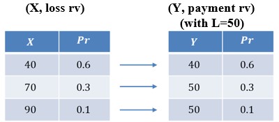
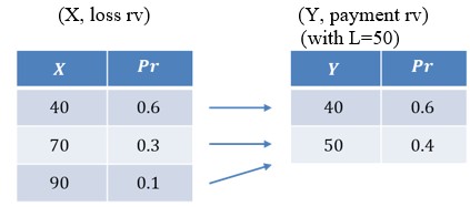
An insurance policy has a loss random variable, \(X\), given in the table below. A policy limit of L=50 is imposed on the policy.

For the second table, since we have 50 twice, we can actually combine them so that the table reduces to:

Like before, we can define \(Y\) as a piecewise function,
$$ Y=\text{Min}\left(X,50\right)=\left\{ \begin{matrix} X, & \text{if } X \lt 50 \\ 50, & \text{if } X \ge 50 \end{matrix} \right. $$
Which can also be expressed as
$$ Y=X \land 50=\text{Min}\left(X,50\right)=\left\{ \begin{matrix} X, & \text{if } X \lt 50 \\ 50, & \text{if } X \ge 50 \end{matrix} \right. $$
Where \(X \land 50\) is read as \(X\) ‘hat’ 50.
$$
{(X-x)}_+= \left\{ \begin{matrix} 0 & \text{if } X \lt x \\ X-x & \text{if } X \ge x \end{matrix} \right. $$
$$ \left(X\land x\right)=\left\{ \begin{matrix} X & \text{if } X \lt x \\ x & \text{if } X \ge x \end{matrix} \right. $$
If we add these two together, we get \(X\), i.e.,
$$ \begin{align*} X & ={(X-x)}_++\ (X\land x) \\
\Rightarrow E\left[X\right]& =E\left[\left(X-x\right)_+\right] +E[\left(X\land x\right)] \\
\Rightarrow E\left[\left(X-x\right)_+\right] & =E\left[X\right]-E[\left(X\land x\right)] \end{align*} $$
We can also use an alternative method to carry out calculations concerning policy limits. In an attempt to further reduce the payment random variable \(Y\), insurance companies may cap the covered loss at a given level C, where C is less than the maximum possible loss B.
In this scenario, the relationship between \(Y\) and \(X\) can be expressed as follows:
$$ Y=\left\{ \begin{matrix} X & \text{if } A \le X \lt C \\ C & \text{if } C \le X \lt B \end{matrix} \right. $$
$$ \begin{align*}
\Rightarrow E\left[Y\right] & =\int_{A}^{C}{x \cdot f_x\left(x\right)dx+}\int_{C}^{B}{C\cdot f_x\left(x\right)dx} \\ & =\int_{A}^{C}{x \cdot f_x\left(x\right)dx+}C\int_{C}^{B}{ f_x\left(x\right)dx} \end{align*} $$
We can also express the expectation of \(Y\) as follows:
$$ E\left[Y\right]=\int_{A}^{C}{x \cdot f_x\left(x\right)dx+}CPr(X \gt C) $$
In a medical life insurance offered by a Canadian firm, the loss amount takes on a uniform distribution with the following density:
$$ f_x\left(x\right)=\frac{1}{5,000};\ \ 0\le x\le 5,000 $$
Assuming a benefit cap of CAD 1,000 and a deductible of zero apply for every loss, calculate the expected claim.
Solution
If \(Y\) is the payment (payout), Let \(X\) be the loss amount random variable, and \(Y\) be the payment per loss random variable.
$$ Y= \left\{ \begin{matrix} X & \text{if } 0 \le X \lt 1,000 \\ 1,000 & \text{if } 1,000 \le X \lt 5,000 \end{matrix} \right. $$
Therefore,
$$ \begin{align*} E\left[Y\right] & =\int_{A}^{C}{x \cdot f_x\left(x\right)dx+}C\int_{C}^{B}{\ f_x\left(x\right)dx} \\ & =\int_{0}^{1,000} x \cdot f_x (x)dx+1,000 \int_{1,000}^{5,000} f_x (x) dx \\
& =\int_{0}^{1,000}{x \left(\frac{1}{5,000}\right)dx+}1,000\int_{1,000}^{5,000}{ \frac{1}{5,000}dx} \\ & =\frac{x^2}{10,000}\vert_0^{1,000}+1,000\left[\frac{x}{5,000}\right]\vert_{1,000}^{5,000} \\
& =100+1,000\left[\frac{5,000}{5,000}-\frac{1,000}{5,000}\right] \\ & =100+1,000\left[\frac{4,000}{5,000}\right]=900
\end{align*} $$
To understand the application of coinsurance and inflation to insurance, consider the following example.
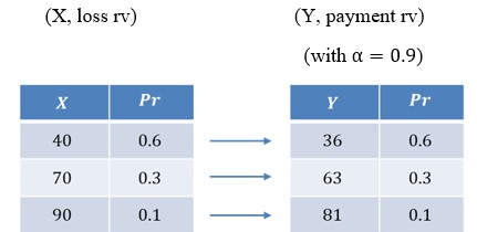
An insurance policy has a loss random variable, \(X\), given in the table below. A coinsurance factor of \(\alpha=0.9\) is imposed on the policy.

Note that to find the payment random variable \(Y\), we take the loss variable multiplied by the coinsurance factor, \(\alpha=0.9\). i.e.,
$$ \begin{align*}
Y & =\alpha\cdot X \\
\Rightarrow E[Y] & =\alpha \cdot E[X] \end{align*} $$
and,
$$ Var(Y)=\alpha^2\cdot Var(X) $$
Losses during the 2023 calendar year follow an exponential distribution with a mean of 1000. Losses during the 2024 calendar year increase over losses during the 2023 calendar year by a 5% inflation rate. Determine the probability that losses during the 2024 calendar year exceed 1500.
Solution
Since losses during the 2023 calendar year follow an exponential distribution with a mean of 1000, we can write,
$$ X_{2023} \sim Exp(\theta=1000) $$
But since we know that,
$$ \begin{align*}
Y & =\alpha \cdot X \\
\Rightarrow {X}_{2024} & =1.05 \cdot X_{2023} \end{align*} $$
We are required to find
$$ \begin{align*} P(X_{2024} \gt 1500) & =P(1.05\times X_{2023} \gt 1500) \\
& =P(X_{2023} \gt \frac{1500}{1.05}) \\
& = Pr(X_{2023} \gt 1428.571\cdots) \\
& =e^{-\left(\frac{1428.571\cdots}{1000}\right)}=0.23965\cdots \end{align*} $$
Summary
Deductibles:
\( Y^L{=(X-d)}_+= \left\{ \begin{matrix} 0,& \text{if }X \le d \\ X-d, & \text{if } X \gt d \end{matrix} \right.\) the payment per loss random variable
\( Y^P=\left(X-d\right)|_{X \gt d} \text{ the payment per payment random variable} \)
$$ \begin{align*} E\left[\left(Y^L\right)^k\right] & =E\left[\left(Y^P\right)^k\right]\cdot Pr(X \gt d) \\
Var(Y^L) & \neq Var(Y^P) \cdot Pr(X \gt d) \end{align*} $$
Policy Limits:
\( Y=X\land L= \left\{ \begin{matrix} X & \text{if } X \le L \\ L & \text{if } X \gt L \end{matrix} \right.\) the payment per loss random variable
$$ \begin{align*} X & =\left(X-x\right)_+ \ + \ \left(X\land x\right) \\
E\left[X\right] & =E[\left(X-x\right)_+] + E[X \land x] \end{align*} $$
Coinsurance \((\alpha \lt 1)\) and Inflation \((\alpha \gt 1)\):
$$ Y=Αx $$
An oil distribution company purchases an insurance cover to protect against losses caused by fire. The insurance policy offers no compensation for the first fire incident in a year, but for subsequent fire incidents, it provides a payout of $7,500 each until the end of the year. The annual occurrence of fire incidents, which could result in losses, follows a Poisson distribution with a mean of 1.8. Determine the expected payout that the oil distribution company could receive through this insurance policy over the course of one year.
Solution:
Let \(X\) be the random variable representing the number of such fire incidents per year.
Given that the annual count of fire incidents follows a Poisson distribution with a mean of 1.8, we have:
$$ X \sim P(\lambda=1.8) $$
It’s worth noting that the insurance policy doesn’t offer any compensation for the first fire incident but pays $7,500 for each subsequent incident. If we let Y be the payment random variable, then \(X\) and \(Y\) are related as follows:
$$ \begin{array}{c|c}
\bf X & \bf Y \\ \hline
0 & 0 \\ \hline
1 & 0 \\ \hline
2 & \$7500 \\ \hline
3 & \$15000 \\ \hline
\vdots & \vdots
\end{array} $$
Using the notations developed for policy adjustments, we can express this relationship as:
$$ \begin{align*}
Y & =7500\cdot {(X-1)}_+ \\
\Rightarrow E[Y] & =7500 \cdot E[(X-1)_+]
\end{align*} $$
Recall that, \({E[(X-1)}_+]=EX-E[X\land 1] \)
Recall also \(E\left[X\land 1\right]=\text{Min}(X,1) \)
$$ \begin{array}{c|c}
\bf{{E}[{X}\land {1}]} & \bf{Pr} \\ \hline
0 & P\left(X=0\right)=e^{-1.8} \\ \hline
1 & P(X \geq 1)=1 – e^{-1.8} \end{array} $$
$$ \Rightarrow E[X \land 1]= 1-e^{-1.8} $$
Hence,
$$ \begin{align*} {E[(X-1)}_+] & =E[X]-E[X \land 1] \\
& =1.8-\left(1-e^{-1.8}\right)=0.9653
\end{align*} $$
With the relationship \(E[Y]=7500\cdot E[(X-1)_+]\), the expected payout to the oil distribution company through this insurance policy for one year amounts to:
$$ E[Y]=7500 \cdot E[(X-1)_+]=\$7,500 \times 0.9653\ldots = \$7,239.75 $$
Ground-up losses, \(X\), follow an exponential distribution with a mean of 1000. A deductible of \(d=100\) is imposed. Determine \(E\left[{X|}_{X\geq 100}\right]\)
Solution
$$ \begin{align*} X\sim \text{Exp}\left(\theta\right)\Rightarrow & Y^P={(X-d)|}_{X\geq d}\sim \text{Exp}(\theta) \\
E\left[{X|}_{X\geq 100}\right] & =E\left[({X-100+100)|}_{X\geq 100}\right] \\
& =E\left[({X-100)|}_{X\geq 100}\right]+E\left[{100|}_{X\geq 100}\right] \\
& =E\left[({X-100)|}_{X\geq100}\right]+100 \\
& =1000+100=1100 \end{align*} $$
Notice that the first term above is \(E\left[({X-100)|}_{X\geq 100}\right]\), is the expected value of the payment per payment random variable, and since we know that \(X\) follows an exponential distribution with a mean of 1000, then by the memoryless property of the exponential distribution,
$$ E\left[({X-100)|}_{X\geq 100}\right]=1000 $$
Notice also the second term, \(E\left[{100|}_{X\geq 100}\right]\) is the expected value of a constant, and therefore, the answer will still be the constant. It doesn't matter whether the distribution is conditional or not.
Alternate (Direct) Solution: \(E\left[{X|}_{X\geq 100}\right]=\int_{100}^{\infty} {x\cdot f_{{X|}_{X\geq 100}}\left(x\right)}dx \)
Fact: Given \(f_X(x)\), the density function for \(X\), then the density function for \({X|}_E\) is
$$ \begin{align*}
f_{{X|}_E}\left(x\right) & =\frac{f_X(x)}{Pr(E)} \text{ for } x^\prime \text{ which make E true} \\
\therefore f_{{X|}_{X\geq 100}}\left(x\right) & =\frac{f_X(x)}{Pr(X\geq 100)}\ \ \text{for } x\geq 100 \\
X\sim \text{Exp}\left(\theta=1000\right) \Rightarrow f_X\left(x\right) &=\frac{1}{1000}e^\frac{-x}{1000}=0.001e^{-0.001x} \end{align*} $$
And from the exponential distribution, the probability, \(Pr{\left(X\geq 100\right)}\) is the survival function evaluated at 100, i.e., \(S_X\left(100\right)\):
$$ \begin{align*}
\Rightarrow Pr{\left(X\geq 100\right)} & =S_X\left(100\right)=e^\frac{-100}{1000}=e^{-0.1} \\
\therefore f_{{X|}_{X\geq100}}\left(x\right) & =\frac{0.001e^{-0.001x}}{e^{-0.1}}=0.001e^{0.1}e^{-0.001x}\ \ \text{for } x\geq 100
\end{align*} $$
Now, since
$$ \begin{align*}
f_{{X|}_{X\geq100}}\left(x\right) & =0.001e^{0.1}e^{-0.001x},\ \ \text{for } x\geq 100 \\
E\left[{X|}_{X\geq 100}\right] & =\int_{100}^{\infty}{x\cdot 0.001e^{0.1}e^{-0.001x}}dx \\ & =0.001e^{0.1}\int_{100}^{\infty}{x\cdot e^{-0.001x}}dx
\end{align*} $$
To solve \(\int_{100}^{\infty}{x\cdot e^{-0.001x}}dx\), we will have to integrate by parts.
$$ \begin{align*} E\left[{X|}_{X\geq100}\right] & =\int_{100}^{\infty}{x\cdot 0.001e^{0.1}e^{-0.001x}}dx \\ & =0.001e^{0.1}\int_{100}^{\infty}{x\cdot e^{-0.001x}}dx \end{align*} $$
Integrating by parts,
$$ \int u d v=uv-\int v d u $$
$$ \begin{align*} \Rightarrow \int_{100}^{\infty}{x\cdot e^{-0.001x}}dx & =\left[x\times \frac{e^{-0.001x}}{-0.001}\right]_{100}^\infty+\frac{1}{0.001}\int_{100}^{\infty}e^{-0.001x}dx \\
& =90,483.7418+904,837.4180=995321.1598 \\
\therefore E\left[{X|}_{X\geq 100}\right] & =0.001e^{0.1}\int_{100}^{\infty}{x\cdot e^{-0.001x}}dx \\
& =0.001e^{0.1}\times995,321.1598=1100 \end{align*} $$
The amount of a claim that an insurance company pays out follows an exponential distribution with a mean of 1000. A deductible of 100 is imposed on the policy. Determine the expected claim payment from the insurance company.
Solution
\( X\sim \text{Exp}(\theta=1000)\), and we seek \(E\left[Y^L\right]=E[\left(X-100\right)_+]\)
Facts:
$$ E\left[Y^P\right]=1000 $$
$$ Pr{\left(X\geq 100\right)}=e^{-0.1}\Rightarrow E\left[Y^L\right]=1000\cdot e^{-0.1}=904.837\cdots $$
Remark:
$$ \begin{align*} E\left[{(Y^L)}^2\right] & =E\left[{(Y^p)}^2\right]\cdot Pr(X\geq d) \\ & =2\cdot {1000}^2\cdot e^{-0.1}=1,809,674.836\cdots \end{align*} $$
Alternate (Direct) Solution:
\(X \sim \text{Exp}(\theta=1000),\) and we seek \(E\left[Y^L\right]=E[\left(X-100\right)_+]\)
$$ \left(X-100\right)_+ = \left\{ \begin{matrix} 0 & \text{if } X \lt 100 \\ X-100 & \text{if } X \geq 100 \end{matrix} \right. $$
$$ \begin{align*}
E\left[Y^L\right] &=\int_{0}^{100}{0\cdot f_X(x)}dx+\int_{100}^{\infty}{(x-100)\cdot f_X(x)}dx \\
& =\int_{100}^{\infty}{(x-100)\cdot 0.001e^{-0.001x}}dx=904.837\cdots
\end{align*} $$
The amount of a claim that an insurance company pays out follows an exponential distribution with a mean of 1000. A deductible of 100 is imposed on the policy. Determine the expected claim payment from the insured.
Solution
\(X \sim \text{Exp}\left(\theta=1000\right)\) and we seek \(E[(X\land 100)]\)
Facts:
\(\begin{align*} X={(X-d)}_+\ +\ (X\land d) & \Rightarrow \left(X\land 100\right)=X-{(X-100)}_+ \\
& \Rightarrow E\left[\left(X\land 100\right)\right]=E\left[X\right]-E[{(X-100)}_+] \\
& \Rightarrow E\left[\left(X\land 100\right)\right]=1000-E\left[Y^L\right] \end{align*} \)
\(E\left[Y^L\right]=E\left[Y^P\right]\cdot Pr\left(X\geq d\right)\) and \(Y^P\sim Exp[\theta=1000]\) and \(P(X \ge 100)=e^{-0.1}\)
\(\Rightarrow E\left[Y^L\right]=1000\cdot e^{-0.1}\)
$$ \therefore E\left[\left(X\land 100\right)\right]=1000-1000\cdot e^{-0.1}=95.162\cdots $$
Alternate (Direct) Solution:
\( X \sim \text{Exp}(\theta=1000),\) and we seek \(E[(X\land 100)]\)
We know that,
$$ \begin{align*}
\left(X\land 100\right) & = \left\{ \begin{matrix} X & \text{if } X \lt 100 \\ 100 & \text{if } X\ge 100 \end{matrix} \right. \\
\Rightarrow E\left[X\land 100\right] & =\int_{0}^{100}{x\cdot f_X(x)}dx+\int_{100}^{\infty}{100\cdot f_X(x)}dx \\
& =\int_{0}^{100}{x\cdot f_X(x)}dx+\int_{100}^{\infty}{100\cdot f_X(x)}dx \\
& =\int_{0}^{100}{x\cdot {0.001e}^{-0.001x}}dx+100\cdot Pr{\left(X \gt 100\right)} \end{align*} $$
Integrating by parts, we get
$$ \Rightarrow E\left[X\land 100\right]=95.162\cdots $$
Ground-up losses, \(X\), follow a uniform distribution over the interval (0,1000). A deductible of \(d=100\) is imposed. Determine \(E[X|_{X\geq 100}]\)
Solution:
Fact:
$$ X \sim U\left(0,\omega\right)\Rightarrow Y^P={(X-d)|}_{X\geq d} \sim U(0,\omega-d) $$
Since \(X\) is uniform over (0,1000),
$$ \begin{align*}
X \sim U\left(0,1000\right) & \Rightarrow{(X-100)|}_{X\geq 100} \sim U(0, 900) \\
E\left[{X|}_{X\geq 100}\right] & =E\left[({X-100+100)|}_{X\geq 100}\right] \\
& =E\left[({X-100)|}_{X\geq 100}\right]+100 \\
& =450+100=550 \end{align*} $$
Remark: \(If X \sim U(a, b)\), then \(E\left(X\right)=\frac{a+b}{2}\)
$$ \Rightarrow E\left[({X-100)|}_{X\geq 100}\right]=\frac{0+900}{2}=450 $$
Alternate (Direct) Solution: \(E\left[{X|}_{X\geq 100}\right]=\int_{100}^{\infty}{x\cdot f_{{X|}_{X\geq 100}}\left(x\right)}dx\)
Where:
$$ \begin{align*}
f_{{X|}_{X\geq 100}}\left(x\right) & =\frac{f_X(x)}{Pr(X\geq 100)}\ \ \text{for}\ x\geq 100 \\
& =\frac{\left(\frac{1}{1000}\right)}{0.9}=\frac{1}{900}\ \ \text{for}\ 100\le x \lt 1000 \\
{\Rightarrow X|}_{X\geq 100} &\sim U(100, 1000) \\
\therefore E\left[{X|}_{X\geq 100}\right] & =\int_{100}^{1000}{x\cdot \frac{1}{900}}dx=\frac{1}{900}\cdot {\frac{x^2}{2}\vert}_{100}^{1000}=550
\end{align*} $$
The amount of a claim that an insurance company pays out follows a uniform distribution over the interval (0,1000). A deductible of 100 is imposed on the policy. Determine the expected claim payment from the insurance company.
Solution: \(X \sim U(0,1000)\), and we seek \(E\left[Y^L\right]=E[\left(X-100\right)_+]\)
Facts:
$$ X \sim U\left(0,1000\right) \Rightarrow Y^P={(X-100)|}_{X\geq 100} \sim U\left(0,900\right) $$
$$ E\left[Y^P\right]=450 $$
$$ Pr{\left(X\geq100\right)}=\frac{900}{1000}=0.9\Rightarrow E\left[Y^L\right]=450\cdot 0.9=405 $$
Remark: \(E\left[{(Y^L)}^2\right]=E\left[{(Y^p)}^2\right]\cdot Pr(X\geq d)=\left(\frac{{900}^2}{12}+{450}^2\right)\cdot 0.9=243,000\)
Note, for a uniformly distributed random variable, \(X\), \(Var\left(X\right)=\frac{\left(b-a\right)^2}{12}\).
Alternate (Direct) Solution: \(X \sim U(0,\omega=1000)\), and we seek \(E\left[Y^L\right]=E[\left(X-100\right)_+]\)
$$
\left(X-100\right)_+= \left\{ \begin{matrix} 0 & \text{if }X\lt 100 \\ X-100 & \text{if }X\geq 100 \end{matrix} \right. $$
$$ \begin{align*}
\Rightarrow E\left[Y^L\right] &=E\left[\left(X-100\right)_+\right] \\ &=\int_{0}^{100}{0\cdot f_X(x)}dx+\int_{100}^{1000}{(x-100)\cdot f_X(x)}dx \\
& =\int_{100}^{1000}{(x-100)\cdot 0.001}dx=405 \end{align*} $$
The amount of a claim that an insurance company pays out follows a uniform distribution over the interval (0,1000). A deductible of 100 is imposed on the policy. Determine the expected claim payment from the insured.
Solution: \(X \sim U(0,\omega=1000)\), and we seek \(E[(X\land 100)]\)
Facts:
$$ \begin{align*} \Rightarrow E\left[\left(X\land 100\right)\right] & =E\left[X\right]-E[{(X-100)}_+] \\
\Rightarrow E\left[\left(X\land100\right)\right] & =500-E\left[Y^L\right] \end{align*} $$
$$ \therefore E\left[\left(X\land 100\right)\right] =500-405=95 $$
Alternate (Direct) Solution: \(X \sim U(0,\omega=1000)\), and we seek \(E[(X\land 100)]\)
$$ \left(X\land 100\right)= \left\{ \begin{matrix} X & \text{if }X \lt 100 \\ 100 & \text{if }X \geq 100 \end{matrix} \right. $$
$$ \begin{align*} \therefore E\left[X\land100\right] & =\int_{0}^{100}{x\cdot f_X(x)}dx+\int_{100}^{1000}{100\cdot f_X(x)}dx \\
& =\int_{0}^{100}{x\cdot 0.001}dx+100\cdot Pr(X \gt 100) \\
& =0.001\int_{0}^{100}xdx+100\cdot 0.9 \\
& =5+90=95 \end{align*} $$
Question
In a medical life insurance offered by a Canadian firm, the loss amount takes on a uniform distribution with the following density:
$$ f_x\left(x\right)=\frac{1}{10,000};\ \ 0\le x\le 10,000 $$
Assume a deductible of CAD 1,000 applies for every loss.
Calculate the expected loss, \(X\)
- 7,500
- 1,000
- 2,500
- 10,000
- 5,000
Solution
The correct answer is D.
Let \(X\) be the loss random variable, \(Y\) be the payment per loss random variable with a deductible of \(d=1000\).
We know that:
$$ \begin{align*} E\left[X\right] &=\int_{A}^{B}{xf_x\left(x\right)}dx \\ & =\int_{0}^{10,000}x\left(\frac{1}{10,000}\right)dx \\ & =\left(\frac{1}{10,000}\right)\left(\frac{x^2}{2}\right)\vert\begin{matrix}10,000\\x=0\\\end{matrix}=10,000
\end{align*} $$
Learning Outcome
Topic 2.f: Univariate Random Variables – Calculate the expected value, variance, and standard deviation of both the loss random variable and the corresponding payment random variable upon the application of policy adjustments.
Get Ahead on Your Study Prep This Cyber Monday! Save 35% on all CFA® and FRM® Unlimited Packages. Use code CYBERMONDAY at checkout. Offer ends Dec 1st.