T-distribution

The student’s T-distribution is a bell-shaped probability distribution symmetrical about its mean. It is considered the best distribution to use for the construction of confidence intervals when:

1. dealing with small samples of less than 30 elements;
2. the population variance is unknown; and
3. the distribution involved is either normal or approximately normal.

In the absence of outright normality of a given distribution, the T-distribution may still be appropriate for use if the sample size is large enough to allow the application of the central limit theorem. In this case, the distribution is considered approximately normal.

The T-statistic, also called the T-score, is given by:

$$ t = \cfrac {(x – \mu)}{\left(\cfrac {S}{\sqrt n} \right)} $$

Where:

x is the sample mean,

μ is the population mean,

S is the sample standard deviation,

n is the sample size.

The T-distribution allows us to analyze distributions that are not perfectly normal. It has the following properties:

1. it has a mean of zero;
2. its \(\text {variance}= \frac {v}{ \left(\frac {v}{2} \right) }\), where v represents the number of degrees of freedom and v ≥ 2;
3. although it’s very close to one when there are many degrees of freedom, the variance is greater than 1 at all times. With a large number of degrees of freedom, the T-distribution resembles the normal distribution; and
4. its tails are fatter than those of the normal distribution, indicating more probability in the tails.

The Degrees of Freedom

The T-distribution, just like several other distributions, has only one parameter: the degrees of freedom (d.f.). The number of degrees of freedom refers to the number of independent observations (total number of observations less 1):

$$ v = n-1 $$

Hence, a sample of 10 observations or elements would be analyzed using a T-distribution with 9 degrees of freedom. Similarly, a 6 d.f. distribution would be used for a sample size of 7 observations.

Notations

It is standard practice for statisticians to use t_α to represent the T-score with a cumulative probability of (1 – α). Therefore, if we were interested in a T-score with a 0.9 cumulative probability, α would be equal to 1 – 0.9 = 0.1. We would denote the statistic as t_0.1.

However, the value of t_α depends on the number of degrees of freedom. For example,

\(t_{0.05,2}= 2.92\) where the second subscript (2) represents the number of d.f., and

$$ t_{0.05,20} = 1.725 $$

Important Relationships

$$ t_{\alpha}= -t_{1 – \alpha} \text{ and } t_{1 – \alpha} = -t_{\alpha} $$

The above relationships are true because the T-distribution is symmetrical about the mean.

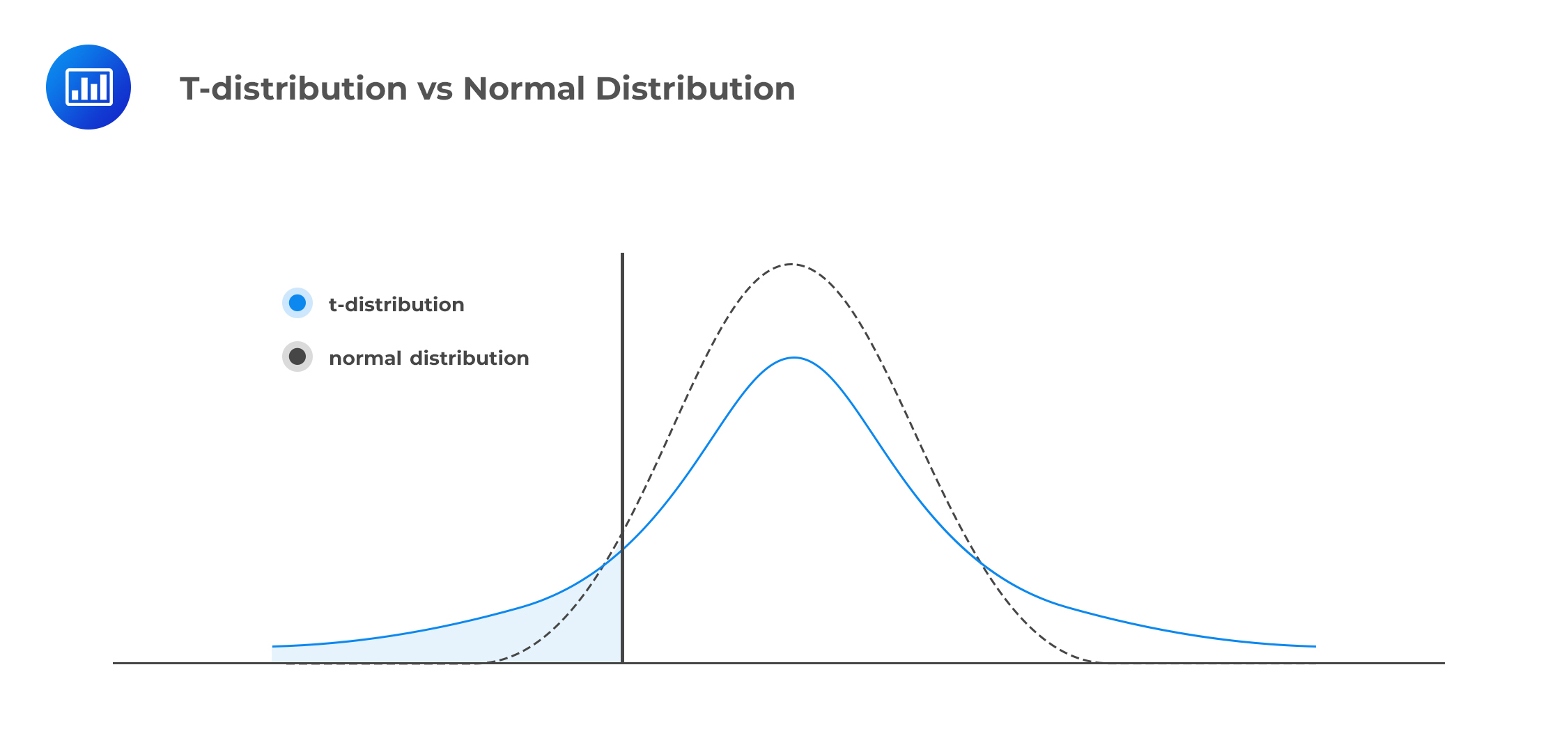
The T-distribution has thicker tails relative to the normal distribution.

The shape of the T-distribution is dependent on the number of degrees of freedom so that as the number of d.f. increases, the distribution becomes more ‘spiked,’ and its tails become thinner.

The table below represents one-tailed confidence intervals and various probabilities for a range of degrees of freedom.

$$ \begin{array}{c|c|c|c|c} \textbf{r} & \textbf{90%} & \textbf{95%} & \textbf{97.5%} & \textbf{99.5%} \\ \hline {1} & {3.07768} & {6.31375} & {12.7062} & {63.6567} \\ \hline {2} & {1.88562} & {2.91999} & {4.30265} & {9.92484} \\ \hline {3} & {1.63774} & {2.35336} & {3.18245} & {5.84091} \\ \hline {4} & {1.53321} & {2.13185} & {2.77645} & {4.60409} \\ \hline {5} & {1.47588} & {2.01505} & {2.57058} & {4.03214} \\ \hline {10} & {1.37218} & {1.81246} & {2.22814} & {3.16927} \\ \hline {30} & {1.31042} & {1.69726} & {2.04227} & {2.75000} \\ \hline {100} & {1.29007} & {1.66023} & {1.98397} & {2.62589} \\ \hline {\infty} & {1.29007} & {1.66023} & {1.98397} & {2.62589} \\ \end{array} $$