Bayes’ Formula
Bayes’ formula is used to calculate an updated or posterior probability given a... Read More
The decision rule refers to the procedure followed by analysts and researchers when determining whether to reject or not to reject a null hypothesis. We use the phrase “not to reject” because it is considered statistically incorrect to “accept” a null hypothesis. Rather, we can only assemble enough evidence to support it.
The decision to either reject or not to reject a null hypothesis is guided by the distribution the test statistic assumes. This means that if the variable involved follows a normal distribution, we use the level of significance of the test to come up with critical values that lie along the standard normal distribution.
Note that before one makes a decision to reject or not to reject a null hypothesis, one must consider whether the test should be one-tailed or two-tailed. This is because the number of tails determines the value of α (significance level). The following is a summary of the decision rules under different scenarios.
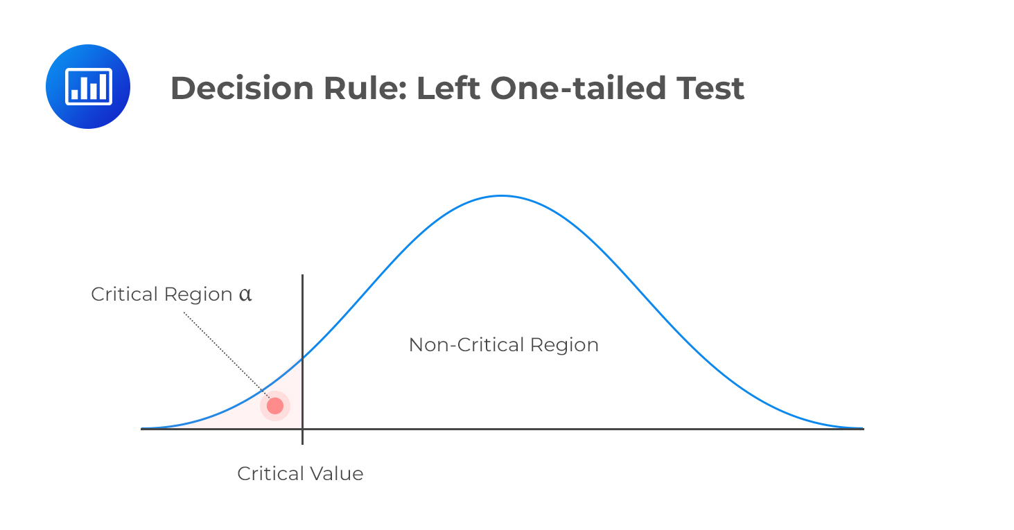
H1: Parameter < X
Decision rule: Reject H0 if the test statistic is less than the critical value. Otherwise, do not reject H0.

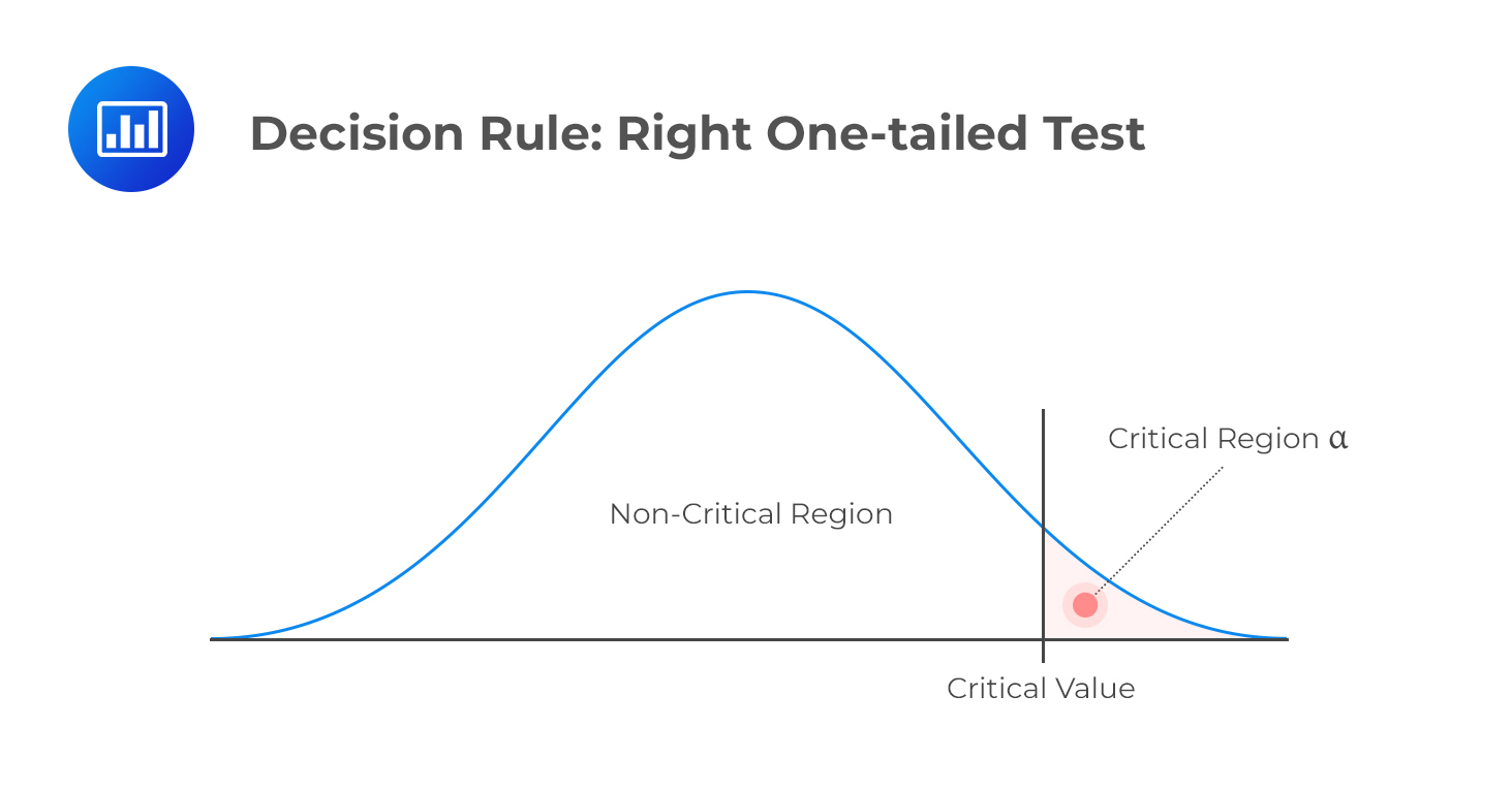
H1: Parameter > X
Decision rule: Reject H0 if the test statistic is greater than the critical value. Otherwise, do not reject H0.

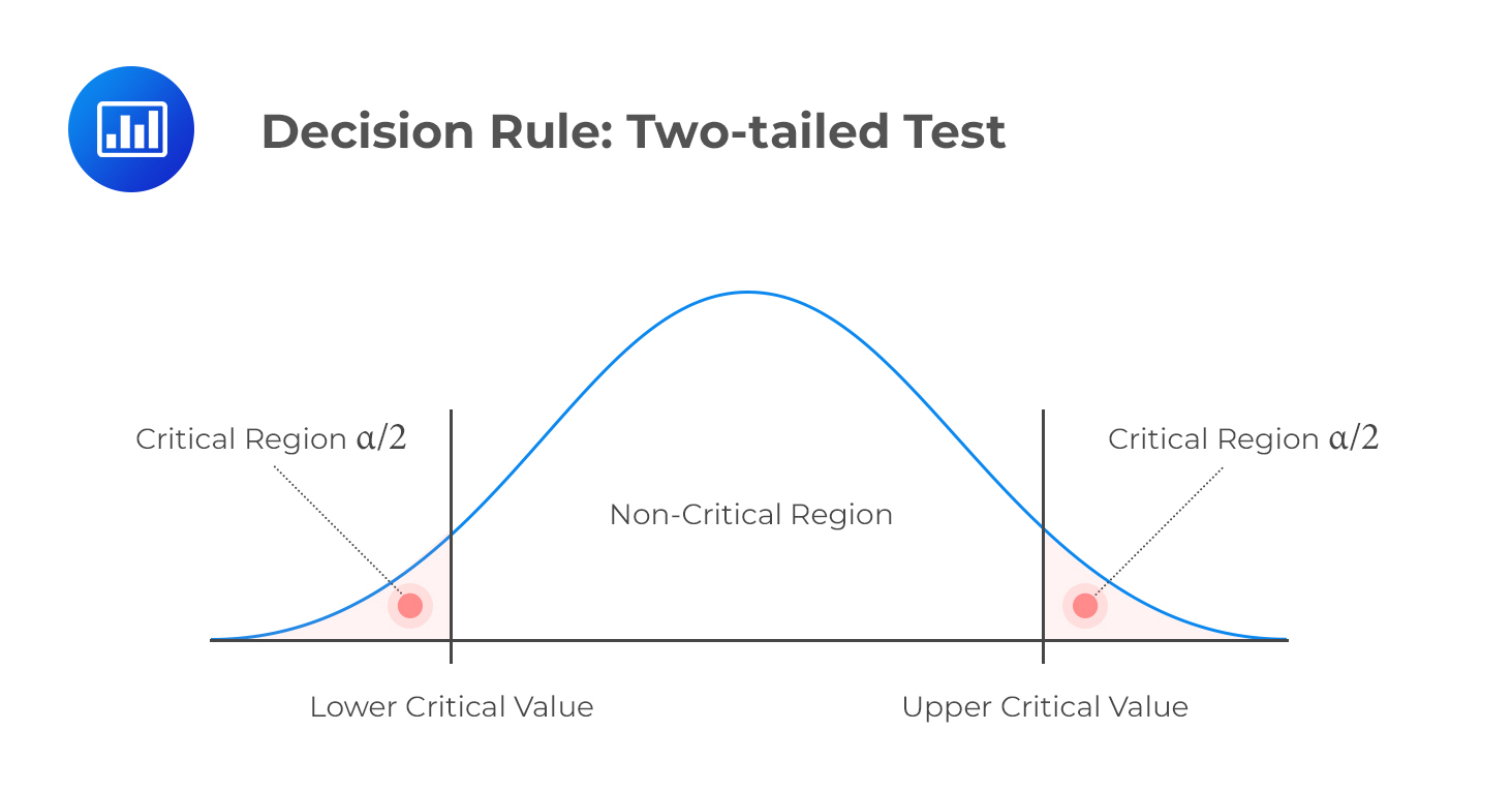
H1: Parameter ≠ X (not equal to X)
Decision rule: Reject H0 if the test statistic is greater than the upper critical value or less than the lower critical value.

Critical values link confidence intervals to hypothesis tests. For example, to construct a 95% confidence interval assuming a normal distribution, we would need to determine the critical values that correspond to a 5% significance level. Similarly, if we were to conduct a test of some given hypothesis at the 5% significance level, we would use the same critical values used for the confidence interval to subdivide the distribution space into rejection and non-rejection regions.
A survey carried out using a sample of 50 Level I candidates reveals an average IQ of 100. Assuming that IQs are distributed normally, carry out a statistical test to determine whether the mean IQ is greater than 105. You are instructed to use a 5% level of significance. (Previous studies give a standard deviation of IQs of approximately 20.)
Solution
First, state the hypothesis:
H0: μ = 105 vs H1: μ > 105
Since IQs follow a normal distribution, under \(H_0, \frac {(X’ – 100)}{\left( \frac {\sigma}{\sqrt n} \right)} \sim N(0,1)\).
Next, we compute the test statistic, which is \(\frac {(105 – 100)}{\left(\frac {20}{\sqrt {50}} \right)} = 1.768\).
This is a right one-tailed test, and IQs are distributed normally. Therefore, we should compare our test statistic to the upper 5% point of the normal distribution.
From the normal distribution table, this value is 1.6449. Since 1.768 is greater than 1.6449, we have sufficient evidence to reject the H0 at the 5% significance level. Therefore, it is reasonable to conclude that the mean IQ of CFA candidates is greater than 100.
(Note the choice of words used in the decision-making part and the conclusion.)
Statistical significance refers to the use of a sample to carry out a statistical test meant to reveal any significant deviation from the stated null hypothesis. We then decide whether to reject or not reject the null hypothesis.
Economic significance entails the statistical significance and the economic effect inherent in the decision made after data analysis and testing.
The need to separate statistical significance from economic significance arises because some statistical results may be significant on paper but not economically meaningful. The difference from the hypothesized value may carry some statistical weight but lack economic feasibility, making implementation of the results very unlikely. Perhaps an example can help you gain a deeper understanding of the two concepts.
A well-established pharmaceutical company wishes to assess the effectiveness of a newly developed drug before commercialization. The company’s board of directors commissions a pilot test. The drug is administered to a few patients to whom none of the existing drugs has been prescribed. A statistical test follows and reveals a significant decrease in the average number of days taken before full recovery. The company considers the evidence sufficient to conclude that the new drug is more effective than existing alternatives.
However, the production of the new drug is significantly more expensive because of the scarcity of the active ingredient. Furthermore, the company would have to engage in a year-long lobbying exercise to convince the Food and Drug Administration and the general public that the drug is indeed an improvement to the existing brands. At the end of the day, the management decides to delay the commercialization of the drug because of the higher production and introduction costs.
Other factors that may affect the economic feasibility of statistical results include:
Evidence of returns based solely on statistical analysis may not be enough to guarantee the implementation of a project. In particular, large samples may produce results that have high statistical significance but very low applicability.
Question
Use data from the previous example to carry out a test at 5% significance to determine whether the average IQ of candidates is greater than 102.
- There is sufficient evidence to justify the rejection of the H0 and inform the conclusion that the average IQ is greater than 102.
- There is insufficient evidence to justify the rejection of the H0 and guide the conclusion that the average IQ is not more than 102.
- There is sufficient evidence to justify the rejection of the H0 and inform the conclusion that the average IQ is greater than 102.
Solution
The correct answer is B.
Just like in the example above, start with the statement of the hypothesis;
H0: μ = 102 vs. H1: μ > 102
The test statistic is \(\frac {(105 – 102)}{\left( \frac {20}{\sqrt{50}} \right)} = 1.061\).
Again, this is a right one-tailed test but this time, 1.061 is less than the upper 5% point of a standard normal distribution (1.6449). Therefore, we do not have sufficient evidence to reject the H0 at the 5% level of significance. It is, therefore, reasonable to conclude that the average IQ of CFA candidates is not more than 102.
Get Ahead on Your Study Prep This Cyber Monday! Save 35% on all CFA® and FRM® Unlimited Packages. Use code CYBERMONDAY at checkout. Offer ends Dec 1st.