Bootstrap Resampling

Resampling

Resampling means repeatedly drawing samples from the original observed sample to make statistical inferences about population parameters. There are two common methods: Bootstrap and jackknife. Here, we’ll focus on the Bootstrap method.

Bootstrap Resampling

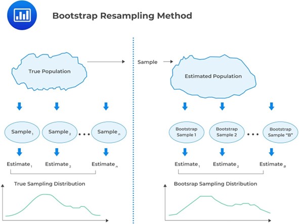
Bootstrap resampling relies on computer simulations for statistical inferences, bypassing the need for conventional analytical formulas like z-statistics. The bootstrap technique is underpinned by a strategy that mirrors the random sampling process from a population to create a sampling distribution.

Note that in bootstrapping, we do not have information about the population. Our only insight comes from a sample of size \(n\) drawn from this “unknown population.”

The core concept is that a random sample can effectively stand in for the entire population. So, we can mimic drawing samples from the population by repeatedly resampling from the initial sample. Essentially, the bootstrap method treats the initially obtained sample as a stand-in for the entire population.

Bootstrapping vs Monte Carlo Simulation

Both bootstrap and Monte Carlo simulation techniques heavily rely on repetitive sampling. Bootstrap considers the resampled dataset a proxy for the true population and infers population parameters such as mean, variance, skewness, and kurtosis from the statistical distribution of these samples.

Conversely, Monte Carlo simulation is centered on the generation of random data with a pre-determined statistical distribution of parameter values.

Simulation Using Bootstrapping

Simulation using bootstrapping is similar to Monte Carlo Simulation except for the source of random variables. In bootstrapping, the random variables are taken from a bootstrap sample instead of a probability distribution.

Consider the previous example:

Let’s say an investor wants to understand the potential outcomes of investing in a portfolio with a 70-30 split between stocks and bonds over a 20-year period. Here’s how a Monte Carlo simulation could be set up.

The simulation steps using the bootstrap sampling distribution are as follows:

Specifying the Simulation

Step 1: Specify the quantity of interest in terms of underlying variables

The quantity of interest here could be the final portfolio value after 20 years, denoted as \(V_{iT}\). The underlying variable is the return on the portfolio. The starting portfolio value is $100,000, with 70% invested in stocks and 30% in bonds.

Step 2: Specify a time horizon

Assume we’re interested in yearly returns, so the time horizon is 20 years. Divide the calendar time into sub-periods. In this case, we will assume yearly returns so that the number of subperiods is \(K = 20\), and time increment \({\Delta t}\) is, therefore, one year.

Step 3: Generate bootstrap samples from the empirical distribution of portfolio returns

Here, we use the historical return data as our empirical distribution. Instead of assuming that the annual portfolio return follows a specific theoretical distribution, we will use the bootstrap procedure to draw the \(K=20\) yearly returns from the observed empirical distribution.

Running the Simulation Over a Given Number of Trials

Step 4: Use the bootstrap samples to produce portfolio values used to value the contingent claim

This step involves using the bootstrap samples drawn in Step 3 to compute the yearly changes in portfolio value. From there, we create a sequence of 20 portfolio values, starting with the initial value of $100,000.

Step 5: Calculate the final portfolio value

The average portfolio value at the end of 20 years \((V_{iT})\) is calculated by summing up the portfolio values at the end of each year and dividing by 20. We then calculate the present value \((V_{i0})\) of this average value by discounting it to the present using an appropriate interest rate. The subscript \(i\) in \(V_{iT}\) and \(V_{i0}\) indicates that these values are from the ith bootstrap sample. This completes one bootstrap sample.

Step 6: Repeat steps 4 and 5 over the required number of trials

Finally, we repeat steps 4 and 5 multiple times, say, 1,000 times. We then calculate summary statistics, such as the mean, median, and percentiles of the distribution of \(V_{i0}\) values. These summary statistics provide a range of potential outcomes for the portfolio value after 20 years, helping the investor understand the risks and rewards of the investment strategy based on the observed empirical distribution of returns.

Question

Which of the following statements is most likely accurate in relation to bootstrap analysis?

1. Bootstrap analysis aims to deduce statistics about population parameters from a singular sample.
2. Bootstrap analysis involves the repeated extraction of samples of equal size, with replacement, from the initial population.
3. During bootstrap analysis, it is necessary for analysts to determine probability distributions for primary risk factors that govern the underlying random variables.

Solution

The correct answer is A.

The bootstrap analysis employs random sampling to generate an observed variable from a set of unknown population parameters. Although the actual distribution of the population is unknown to the analyst, the parameters of the population can be inferred through the sample produced via random sampling.

B is incorrect. In bootstrap analysis, the analyst repeatedly samples from the initial sample, not the entire population. Each resample has the same size as the original sample, and for each new draw, selected items go back into the sample.

C is incorrect. During bootstrap analysis, analysts simply utilize the empirical distribution of the observed underlying variables. In contrast, the analyst must establish probability distributions for the key risk factors that govern the underlying variables in a Monte Carlo simulation.