How IS and LM Curves Combine to Generate the Aggregate Demand Curve

Also known as the Hicks-Hansen model, the IS-LM curve is a macroeconomic tool used to show how interest rates and real economic output relate.

IS refers to Investment-Saving while LM refers to Liquidity preference-Money supply. These curves are used to model the general equilibrium and have been given two equivalent interpretations. First, the IS-LM model explains the changes that occur in national income with a fixed short-run price level. Secondly, the IS-LM curve explains the causes of a shift in the aggregate demand curve.

In the next sections, we will first have an overview of the general IS-LM equilibrium, and then we will describe both curves.

The IS-LM Model

The model is represented as a graph consisting of two intersecting lines. On the X-axis, we have the real gross domestic product (Y), which is simply the output of the economy. On the Y-axis, we have nominal interest rates (i).

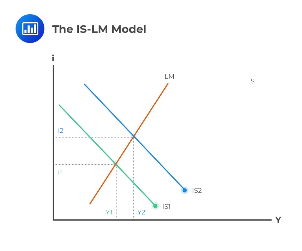
The intersection of the IS and LM curves shows the equilibrium point of interest rates and output when money markets and the real economy are balanced. If we move one of the two curves to the right or the left, the model gives us a new economic output and interest rates.

IS Curve

Here, the interest rate is the independent variable, while income is the dependent variable. Notably, the curve is downward sloping. The IS also shows the locus point where total income equals total spending:

$$Y=C[Y-T(Y)]+I(r)+G+NX(Y)$$

Where:

\(Y\) = income

\(C[Y-T(Y)]\) = consumer spending as an increasing function of disposable income

\(l(r)\) = investment. A decreasing function of interest rates

\(G\) = government expenditure

\(NX(Y)\) = net exports

Example of the IS Curve

The following equations are given for a certain American state:

Consumption function \((C[Y-T(Y)]) = 1,000 + 0.5(Y – T)\)

Investment function \((I(r, Y)) = 100 + 0.1Y – 30r\)

Government spending \((G) = 1000\)

Net export \((NX)=500-0.6Y\)

Tax function \((T(Y))= –100 + 0.3Y\)

Use the equations above to find the equation that best describes the IS curve.

Solution

Using the identity

$$Y = C[Y-T(Y)] + I(r) + G + NX(Y)$$

We have,

$$Y = 1,000 + 0.5(Y – T(Y))+ 100 + 0.1Y – 30r+ 1000+ 500-0.6Y$$

Substitute the tax function and solve for Y. We get,

$$Y=2304.35-26.092r$$

This is the final equation for the IS curve. It summarizes combinations of income and the real interest rate at which income and expenditure are equal; that is, it reflects the goods market.

LM Curve

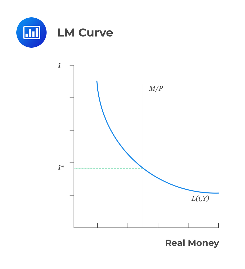
In this case, the independent variable is income, while the dependent variable is interest rates. This curve represents the money market equilibrium. Also, it represents the set of points at an equilibrium between liquidity preference (demand for money) and the money supply function.

By using the quantity of money theory, we get a clear relationship among the nominal money supply (M), the price level (P), and the real income/expenditure (Y):

$$MV=PY$$

Where V is the rate at which the money circulates in the economy (velocity of money). If we assume that V remains constant, then the theory postulates that money supply determines the nominal value of the output (PY). In other words, an increase in the money supply will increase the nominal value of output. However, this equation does not tell us how this increase will be felt in price and quantity.

We can rewrite the quantity theory equation in terms of the supply and demand for real money balance as:

$$M/P=(M/P)_D=kY$$

Where \(k=\frac{1}{V}\) denotes the amount of money people desire to hold for every currency unit of real income. Using the above equation, it’s easy to see that demand for real money balances is inversely proportional to interest rate since high interest rate encourages investors to venture into high-yielding securities. Therefore, the demand for real money balances is an increasing function of real income (M) and a decreasing function of the interest rate.

Equilibrium in a money market requires that:

$$M/P=M(r,Y)$$

By holding the M/P constant, it is easy to see that the real income Y and the real interest rate r have a positive relationship. An increase in income must be followed by an increase in the interest rate so that demand for real money increases balances equal to the supply.

Example of LM Curve

The money demand and supply for a certain American state are:

real Money Demand=\((M/P)_D=-200+0.25Y-30r\); and

real Money Supply=\(M/P=5,000/P\).

Find the equation of the LM curve.

Solution

To find the LM curve, we need to equate the real money supply to real money demand and rearrange it to make Y the subject. That is,

$$(M/P)_D=M/P$$

$$\therefore -200+0.25Y-30r=M/P $$

$$\Rightarrow Y=800+4(M/P) +120r$$

But from the real money supply function, \(M=5,000\). So, the LM equation is,

$$ Y=800+20,000/P +120r $$

Generating the Aggregate Demand Curve

The IS-LM model studies the short run with fixed prices. This model combines to form the aggregate demand curve, which is negatively sloped; hence when prices are high, demand is lower. Therefore, each point on the aggregate demand curve is an outcome of this model.

Aggregate demand occurs at the point where the IS and LM curves intersect at a particular price. If some individual considers a higher price level, then the real supply of money will definitely be lower. As a result, the LM curve will shift higher. Furthermore, the aggregate demand will be lower.

Question

Which of the factors given below is the one whose increase most likely leads to a leftward shift in the aggregate demand curve?

A. Stock prices

B. Business confidence

C. Taxes

Solution

The correct answer is C.

Option A is incorrect. When stock prices increase, the aggregate demand increases due to an increase in consumption.

Option B is also incorrect. An increase in business confidence causes an increase in consumption.

However, an increase in taxes leads to lower consumption. This creates a leftward shift in the aggregate demand curve.