One-Period Binomial Model

The law of arbitrage dictates that the value of any two assets (or portfolio of assets) whose payoffs are identical in all possible future scenarios at a given time must also be identical today. Unlike forward commitments that offer symmetric payoffs at a pre-determined price in the future, contingent claims offer asymmetric payoffs. For this reason, their valuation is a challenge. The binomial model can be used to model the payoffs of contingent claims.

One-Period Binomial Model

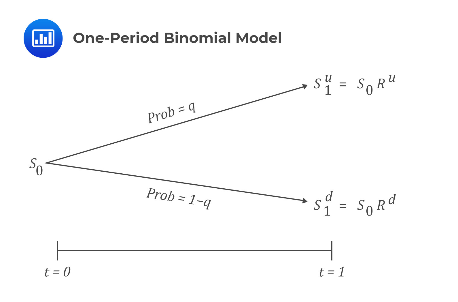
The idea behind the binomial model is that at maturity, an asset’s spot price, \(S_0\), can either increase to \(S_1^u\) or decrease to \(S_1^d\). We do not need to know the asset’s future price in advance since it depends on a random variable’s outcome. The asset price movements, from \(S_0\) to either \(S_1^u\) or \(S_1^d\), can be seen as the outcome of a Bernoulli trial. Let us denote \(q\) as the probability of an increase in the asset’s price. Because of the presence of only two possibilities, i.e., an increase or a decrease in the asset’s price, we can denote the probability of a decrease in its price as \(1-q\), such that the two probabilities will add up to 1. The gross return when the asset price increases will be: $$R^u=\frac{S_1^u}{S_0}>1$$ When the asset price decreases, the gross return will be: $$R^d=\frac{S_1^d}{S_0}<1$$ The difference between \(S_1^u\) (or \(R^uS_o)\) and \(S_1^d\) (or \(R^dS_0\)) is the spread of possible future price outcomes.

Pricing a European Call Option using a One-Period Binomial Model

Consider a one-year call option with an underlying price of \(S_0\) and an exercise price of \(X\). Also, assume that \(S_1^d<X<S_1^u\) and that the one-period binomial model is equivalent to the time of expiration of one year. The one-period binomial model gives the underlying asset values in one year, where the option value is defined as a function of the underlying value.

At time t=0:

The value of the call option is \(c_0\). Note that this value is unknown and needs to be calculated.

At time t=1:

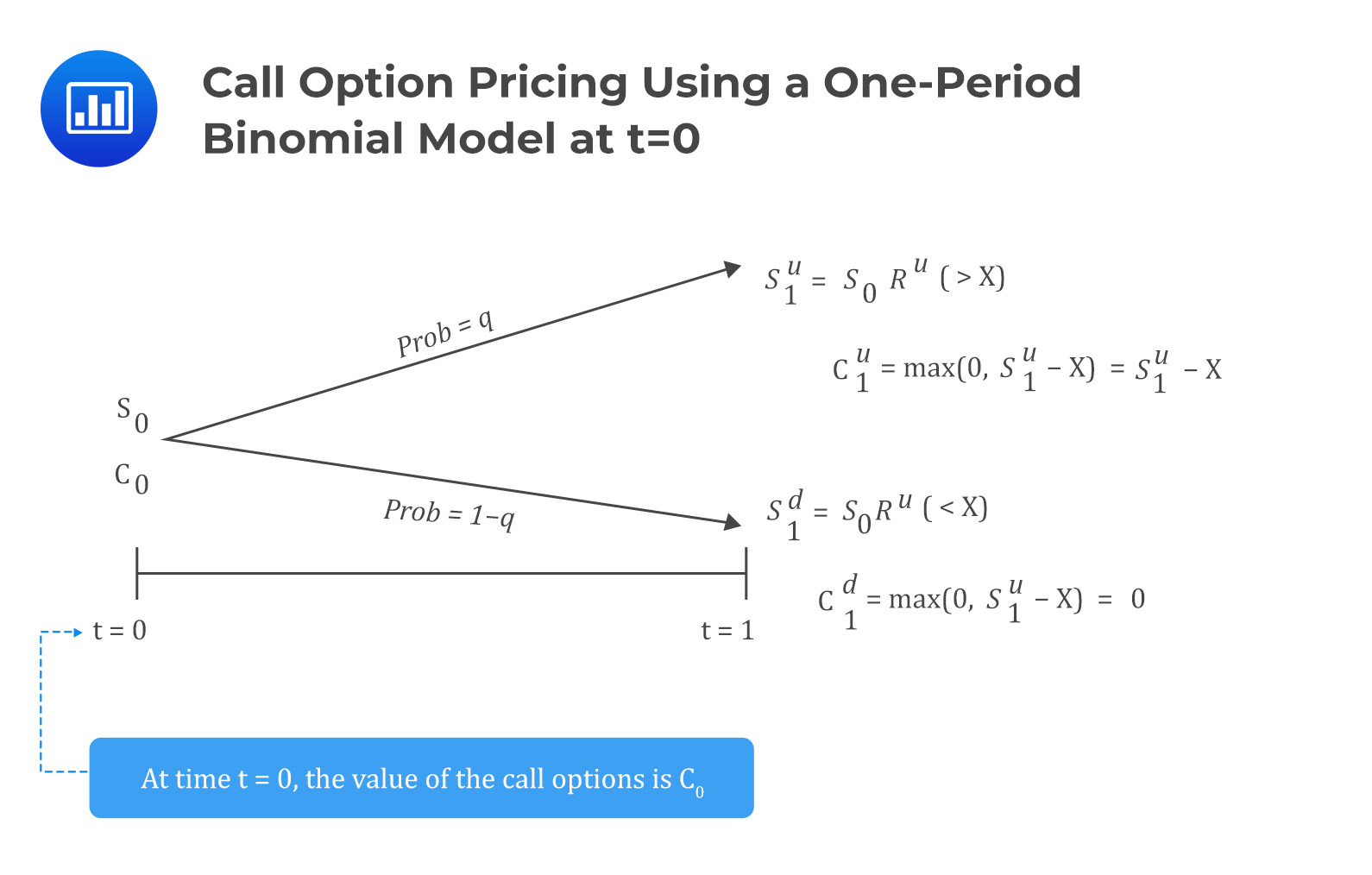
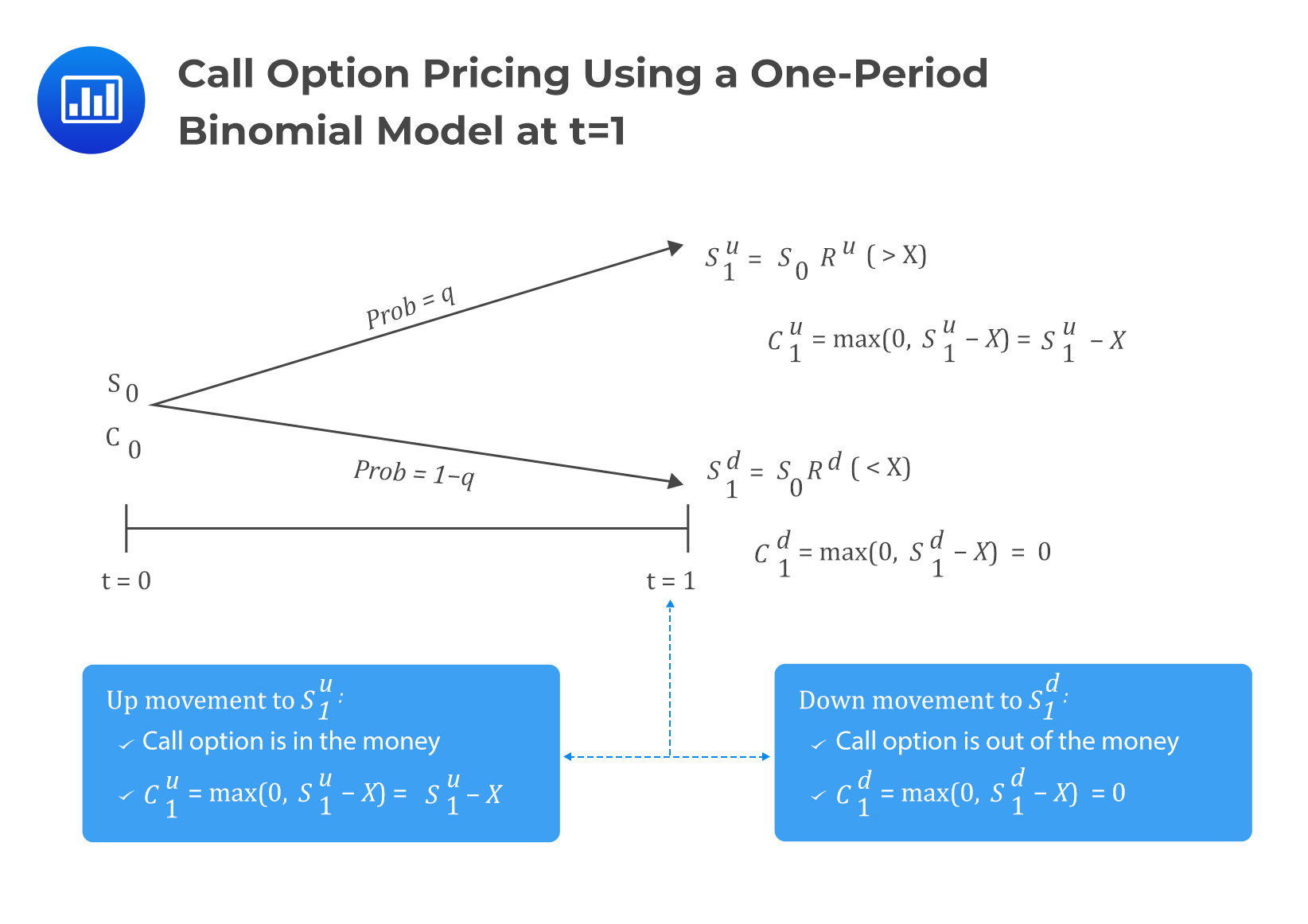
After one year, the option expires. At this time, the value of the option will either be \(c_1^u=\max(0,S_1^u-X)\) if the underlying price rises to \(S_1^u\) or \(c_1^d=\max(0,S_1^u-X)\) if the underlying price falls to \(S_1^d\). Intuitively, for the up movement, the call option is in the money, and for the down direction, the option is out of the money.

Determining the Value of c₀

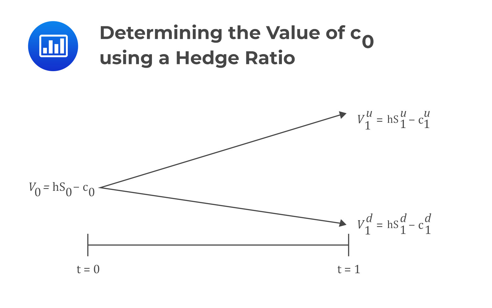
The value of \(c_0\) is determined by applying replication and no-arbitrage pricing. Replication implies that the value of the option and its underlying asset in any future scenario may be used to construct a risk-free portfolio. With that in mind, assume at time \(t=0\), we sell a call option for a price of \(c_0\) and buy \(h\) units of the underlying asset. Also, let the value of the portfolio be \(V\) so that its value at \(t=0\) is: $$V_0={\rm hS}_0-c_0$$ The value of the portfolio, if the underlying price moves up, is given by: $$V_1^u={\rm hS}_1^u-c_1^u=h\times R^u\times S_0-\max{\left(0,S_1^u-X\right)}$$ And for the down movement: $$V_1^d={\rm hS}_1^d-c_1^d=h\times R^d\times S_0-\max{\left(0,S_1^d-X\right)}$$ Assuming no-arbitrage condition, note that we have established two portfolios with identical payoff profiles at time \(t=1\). As such, we need to find the value of \(h\) such that: $$V_1^u=V_1^d$$ Therefore, $$\Rightarrow{hS}_1^u-c_1^u={hS}_1^d-c_1^d$$ Making \(h\) the subject of the formula: $$h=\frac{c_1^u-c_1^d}{S_1^u-S_1^d}$$ The value \(h\) is called the hedge ratio. The hedge ratio is a proportion of the underlying that will offset the risk associated with an option. Since \(V_1^u=V_1^d\), we can draw two conclusions:

• We can utilize either of the two portfolios to value the option.
• The return \(\frac{V_1^u}{V_0}=\frac{V_1^d}{V_0}=1+r\).

To avoid arbitrage, the portfolio value at \(t=1\), (\(V_1={\ V}_1^u=V_1^d\)), must be discounted using a risk-free rate so that: $$V_0=V_1\left(1+r\right)^{-1}$$ However, recall that \(V_0={hS}_0-c_0\): $$\Rightarrow{\rm hS}_0-c_0=V_1\left(1+r\right)^{-1}$$ Making \(c_0\) the subject of the formula: $$c_0={\rm hS}_0-V_1\left(1+r\right)^{-1}$$

Example: Pricing Call Option Using One Period Binomial Model

A European call option that expires in one year has an exercise price of $70 and an underlying spot price of $60. Use a one-period binomial model to estimate the call option price if the underlying’s spot price is expected to change by 25% in one year. Assume that the risk-free annual rate is 5%. Solution Step 1: Determine the Call Option’s Value at Maturity t=1 At maturity, the value can either be \(c_1^u\) if the price of the underlying goes up or \(c_1^d\) if the price of the underlying goes down. The spot price at maturity, if the price goes up by 25%, will be: $$S_1^u=\frac{125}{100}\times60=75$$ and the gross return will be: $$R^u=\frac{S_1^u}{S_o}=\frac{75}{60}=1.25$$ If the price goes down by 25%, the spot price at maturity will be: $$S_1^d=\frac{75}{100}\times60=45$$ and the gross return will be: $$R_d=\frac{S_1^d}{S_o}=\frac{45}{60}=0.75$$ If the underlying’s price goes up (the call option expires in the money): $$c_1^u=\max\ \left(0,\ S_1^u-X\right)=\max\ \left(0,\ 75-70\right)=5$$ If the underlying’s price goes down, and the call option expires out of the money: $$c_1^d=\max\ \left(0,\ S_1^d-X\right)=\max\ \left(0,\ 45-70\right)=0$$ Step 2: Determining h, the Hedge Ratio The hedge ratio is given by $$\begin{align} h&=\frac{c_1^u-c_1^d}{S_1^u-S_1^d}\\&=\frac{5-0}{75-45}=0.167\end{align}$$ The hedge ratio of 0.167 implies that we either need to buy 0.167 units of the underlying for every call option we sell or sell 6 call options for each underlying asset to equate the portfolio values at maturity (\(t=1\)). Therefore, the portfolio values when the price of the underlying increases and decreases respectively is: $$\begin{align}V_1^u&=\left(0.167\times75\right)-5=7.5\\V_1^d&=\left(0.167\times45\right)-0=7.5\end{align}$$ The portfolio values are the same, implying that either of the portfolios can be used to value the derivative. Step 4: Determining \(\mathbf{V_0}\) We can obtain \(V_0\) by discounting \(V_1\) at the risk-free discount rate. Remember that \(V_1=V_1^u=V_1^d\): $$V_o=7.5(1+{0.05)}^{-1}=7.14$$ Step 5: Determining \(\mathbf{c_0}\) Recall that: $$c_0={\rm hS}_0-V_1\left(1+r\right)^{-1}=hS_o-V_0$$ Therefore, $$c_o=hS_o-V_0=\left(0.167\times60\right)-7.14=2.88$$ Note: The hedging approach can be used to value many derivatives, not just call options, provided the derivative’s value depends on the underlying asset’s value at contract maturity, i.e., \(t=1\)

Pricing a European Put Option One-period Binomial Model

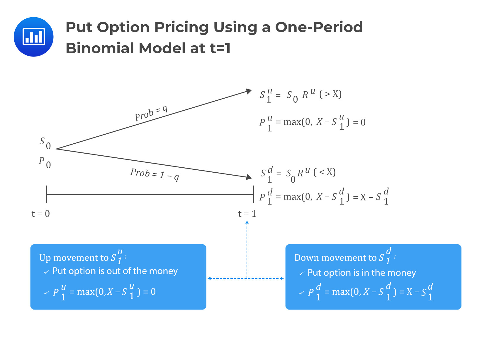
For put options, the same explanations we gave under the call option apply, albeit with a different replication strategy. Consider the following diagram: Under the put option, the hedge ratio is given by $$h=\frac{p_1^u-p_1^d}{S_1^d-S_1^u}$$ Note that the formula remains the same as in the call option, except for the change of notations. Replication in pricing put option using a one-period binomial model involves buying the put option and \(h\) units of the underlying so that: $$V_0=p_0+hS_0$$ Therefore, $$p_0=V_0-hS_0$$

Question

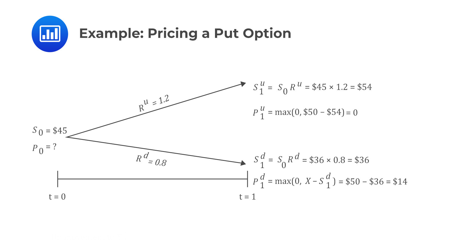
Consider a one-year put option on a non-dividend paying stock with an exercise price of $50. The current stock price is $45. The stock price is expected to go up or down by 20%. Calculate the non-arbitrage price of the put option if the risk-free rate of return is 4%. A. 0 B. $5.38 C. $14.00 Solution The correct answer is B. Consider the following diagram: From the above results, the hedge ratio is given by: $$ h=\frac{p_1^u-p_1^d}{S_1^u-S_1^d}=\frac{0-14}{54-36}=-0.7778 $$ We need to calculate \(V_1={\ V}_1^u=V_1^d\), which are: $$ \begin{align}V_1^u&={\rm hS}_1^u+p_1^u=0.7778\times54+0=\$42.00\\V_1^d&={\rm hS}_1^d+p_1^d=0.7778\times36+14=\$42.00\end{align} $$ Next, we can either use \(V_1^u\) or \(V_1^d\) to calculate the value of \(V_0\): $$ V_0=V_1\left(1+r\right)^{-1}=42\left(1.04\right)^{-1}=\$40.38 $$ Therefore, the put option value is: $$ p_0=V_0-{\rm hS}_0=40.38-0.7778\times45=\$5.38 $$