Hypothesis Tests of Risk and Risk

Hypothesis Test Concerning Single Mean

The z-test is the ideal hypothesis test when the sample’s sampling distribution is normally distributed or when the standard deviation is known.

The z-statistic is the test statistic used in hypothesis testing.

Practice Z-tests and hypothesis testing questions free.

Testing \(\bf{H_0: \mu = \mu_0}\) Using the z-test

Given a random sample of size \(n\) from a normally distributed population with mean \(\mu\), variance \(\sigma^2\), and a sample mean \(\bar X\), we can compute the z-statistic as follows:

$$ \text z-\text{statistic} =\cfrac {(\bar{X} – \mu_0)}{\left(\frac {\sigma}{\sqrt n} \right)} $$

Where:

\(\bar{X}\) is the sample mean.

\(\mu_0\) is the hypothesized mean of the population.

\(\sigma\) is the standard deviation of the population.

\(n\) is the sample size.

Once computed, the z-statistic is compared to the critical value corresponding to the test’s significance level. For example, if the significance level is 5%, the z-statistic is screened against the upper or lower 95% point of the normal distribution \((\pm 1.96)\). The decision rule is to reject the H0 if the z-statistic falls within the critical or rejection region.

Example: z-test

Academics carried out a study on 50 former United States presidents and found an average IQ of 135. You are required to carry out a 5% statistical test to determine whether the average IQ of presidents is greater than 130. (IQs are distributed normally, and previous studies indicate that \(\sigma = 25\).)

Solution

Step 1: State the hypothesis:

\(H_0: \mu \le 130\)

\(H_1: \mu \gt 130\)

Step 2: Identify the appropriate t-statistic:

$$ \text z-\text{statistic} =\cfrac {(\bar{X} – \mu_0)}{\left(\frac {\sigma}{\sqrt n} \right)} $$

Assuming the \(H_0\) is true, \(\frac {(\bar{X} – 130)}{\left(\frac {\sigma}{\sqrt n} \right)} \sim N(0,1)\)

Step 3: Specify the level of significance:

This is a right-tailed test. Therefore, we compare our test statistic to the upper 95% point of the standard normal distribution (1.645).

Step 4: State the decision rule:

Reject the null hypothesis if the z-statistic is greater than 1.645.

Step 5: Calculate the test statistic:

The z-statistic is \(\cfrac {(135 – 130)}{\left(\frac {25}{\sqrt {50}} \right)} = 1.414\)

Step 6: Make a decision:

Since 1.414 is less than 1.645, we do not have sufficient evidence to reject the \(H_0\). As such, it would be reasonable to conclude that the average IQ of U.S. presidents is not more than 130.

The t-test

The t-test is based on the t-distribution. The test is appropriate for testing the value of a population mean when:

• \(\sigma\) is unknown.
• The sample size is large (n > 30), and if n < 30, the distribution must be normal or approximately normal.

Testing \(H_0: \mu = \mu_0\) Using the t-test

We compute a t-statistic with \(n – 1\) degrees of freedom as follows:

$$ t_{n-1} = \cfrac {(\bar{X} – \mu_0)}{\left(\frac {s}{\sqrt n} \right)} $$

Where:

\(\bar{X}\) is the sample mean.

\(\mu_0\) is the hypothesized mean of the population.

\(s\) is the standard deviation of the sample.

\(n\) is the sample size.

Example: t-Test

Financial analysts in a certain equatorial country are interested in evaluating the potential impact of rainfall on agricultural investments. They have gathered data on the annual rate of rainfall (cm) over the last 10 years, as shown below:

{ 25, 26, 25, 27, 28, 29, 28, 27, 26, 25 }

Previously, the recorded average rainfall was 23 cm. The analysts want to find out if there’s been an increase in the average rainfall rate, which could impact agricultural investment. Conduct a statistical test at a 5% significance level to investigate this.

Solution

Follow the steps outlined above.

Step 1: State the hypothesis:

As always, you should begin by stating the hypothesis:

\(H_0: \mu \le 23\)

\(H_1: \mu \gt 23\)

Step 2: Identify the appropriate t-statistic:

If we assume that the annual rainfall quantities are distributed normally and recorded independently, then:

$$ \cfrac {(\bar{X} – \mu_0)}{\left(\frac {s}{\sqrt n} \right)} \sim t_{n- 1} $$

Please, confirm that \(\bar{X}= 26.6\) and \(s = 1.43\)

Step 3: Specify the level of significance:

$$ \alpha=5\%\left(\text{right}-\text{tailed}\right) $$

Step 4: State the decision rule:

Reject the null hypothesis if the t-statistic is greater than \(t_{0.05,9} =1.833\)

Step 5: Calculate the test statistic:

Therefore, our t-statistic = \(\cfrac {(26.6 – 23)}{\left(\frac {1.43}{\sqrt {10}}\right)} = 7.96\)

Step 6: Make a decision:

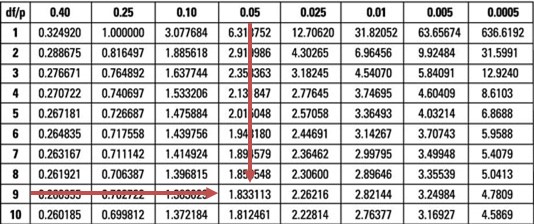
Our test statistic (7.96) is greater than the upper 95% point of the \(t_{0.05,9}\) distribution (1.833).

Therefore, we have sufficient evidence to reject the H0. As such, it is reasonable to conclude that the average annual rainfall has increased from its former long-term average of 23.

Question

What is the value of \(t\) in the example above if the significance level is reduced from 5% to 0.5%, and does this change the decision rule?

1. 2.02; it does not change the decision rule.
2. 3.25; it does not change the decision rule.
3. 3.25; it changes the decision rule.

Solution

The correct answer is B.

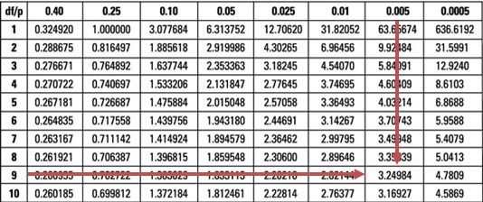
A quick glance at the \(t_{0.005,9}\) distribution when \(\alpha = 0.5\%\) gives a value of 3.25.

However, the evidence against the \(H_0\) is overwhelming since our test statistic (7.96) is still greater than 3.25. As such, the conclusion would remain unchanged.

Hypothesis Test Concerning the Equality of the Population Means

Analysts are often interested in establishing whether there exists a significant difference between the means of two different populations. For instance, they might want to know whether the average returns for two subsidiaries of a given company exhibit a significant variance. Such a test may then be used to make decisions regarding resource allocation or the reward of the directors. Before embarking on such an exercise, ensuring that the samples taken are independent and sourced from normally distributed populations is paramount. It can either be assumed that the population variances are equal or unequal. In this reading, we will assume that the population variances are equal.

Assume that \(\mu_1\) is the mean of the first population while \(\mu_2\) is the mean of the second population. In testing the equality of two population means, we wish to determine whether they are equal. As such, the hypotheses can be any of the following:

1. Two-sided:
   $$H_0: \mu_1 – \mu_2 = 0 \text{ vs. } H_a: \mu_1 – \mu_2 \neq 0,$$This can be stated as follows:
   

   $$H_0: \mu_1 = \mu_2 \text{ vs. } H_a: \mu_1 \neq \mu_2 $$

   
   
2. One-sided (right):
   $$ H_0: \mu_1 – \mu_2 \leq 0 \text{ vs. } H_a: \mu_1 – \mu_2 \gt 0, $$This can be stated as follows:
   

   $$ H_0: \mu_1 \leq \mu_2 \text{ vs. } H_a: \mu_1 \gt \mu_2 $$

   
   
3. One-sided (Left):
   $$ H_0: \mu_1 – \mu_2 \geq 0 \text{ vs. } H_a: \mu_1 – \mu_2 \lt 0, $$This can be stated as follows:
   

   $$ H_0: \mu_1 \geq \mu_2 \text{ vs. } H_a: \mu_1 \lt \mu_2 $$

   
   

   However, note that tests such as \(H_0: \mu_1 – \mu_2 =3 \text{ vs. } H_a: \mu_1 – \mu_2 \neq 3\) are valid. The process is similar in both cases.

   
   

Hypothesis Test Concerning Differences between Means With Independent Samples

When testing for the difference between two population means, we assume that the two populations are distributed normally. Further, we assume that they have equal and unknown variances. We always make use of the student’s t-distribution where the test statistic is given by:

$$
t=\frac{\left(\bar{X}_{1}-\bar{X}_{2}\right)-\left(\mu_{1}-\mu_{2}\right)}{\sqrt{\frac{s_{p}^{2}}{n_{1}}+\frac{s_{p}^{2}}{n_{2}}}}=\frac{\left(\bar{X}_{1}-\bar{X}_{2}\right)-\left(\mu_{1}-\mu_{2}\right)}{s_p\left(\sqrt{\frac{1}{n_{1}}+\frac{1}{n_{2}}}\right)}
$$

Where \(s_p^2\) is the pooled estimator of the common variance and is given by:

$$
s_{p}^{2}=\frac{\left(n_{1}-1\right) s_{1}^{2}+\left(n_{2}-1\right) s_{2}^{2}}{n_{1}+n_{2}-2}
$$

Also, the variables are defined as follows:

\(\bar{X}_1\) = Mean of the first sample.

\(\bar{X}_2\) = Mean of the second sample.

\(s_1^2\) = variance of the first sample.

\(s_2^2\) = variance of the second sample.

\(n_1\) = Sample size of the first sample.

\(n_2\) = Sample size of the second sample.

Example 1: Hypothesis Test Concerning the Equality of the Population Means

Nutritionists want to establish whether obese patients on a new special diet have a lower weight than the control group. After six weeks, the average weight of 10 patients (group A) on the special diet is 75kg, while that of 10 more patients of the control group (B) is 72kg. Carry out a 5% test to determine if the patients on the special diet have a lower weight.

Additional information: \(\sum A^2 = 59,520\) and \(\sum B^2 =56,430 \)

Solution

As is the norm, start by stating the hypothesis:

$$ H_0: \mu_1 – \mu_2 = 0 \text{ Vs } H_a: \mu_1 – \mu_2 \neq 0,$$

We assume that the two samples have equal variances, are independent, and are normally distributed. Then, under \(H_0\),

$$ \frac { \bar { B } -\bar { A } }{ S\sqrt { \frac { 1 }{ m } +\frac { 1 }{ n } } } \sim { t }_{ m+n-2 } $$

Note that the sample variance is given by:

$$s^2=\frac{\sum X^2 -n\bar{X}^2}{n-1}$$

So,

$$ \begin{align*} { S }_{ A }^{ 2 } & =\frac { \left\{ 59520-{ \left( 10\ast { 75 }^{ 2 } \right) } \right\} }{ 9 } =363.33 \\ { S }_{ B }^{ 2 } & =\frac { \left\{ 56430-{ \left( 10\ast { 72}^{ 2 } \right) } \right\} }{ 9 } =510 \\ \end{align*} $$

Therefore,

$$ S^p_2 =\cfrac {(9 \times 363.33 + 9 \times 510)}{(10 + 10 -2)} = 436.665 $$

And

$$ \text{Test statistic} =\cfrac {(75 -72)}{ \left\{ \sqrt{439.665} \times \sqrt{ \left(\frac {1}{10} + \frac {1}{10}\right)} \right\} }= 0.3210 $$

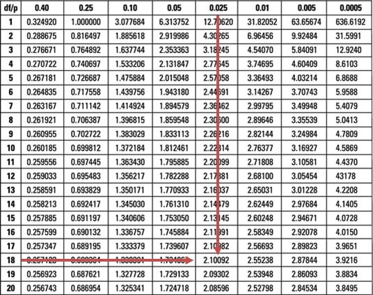
Our test statistic (0.3210) falls within the bounds of the two critical values (\(\pm 2.101\)) of the t-distribution with 18 degrees of freedom.

Therefore, we do not have sufficient evidence to reject the \(H_0\) at 5% significance. As such, it is reasonable to conclude that the special diet has the same effect on body weight as the placebo.

Hypothesis Test Concerning Differences between Means With Dependent Samples

There are some challenges when testing the difference between two population means using independent samples. Variability within each sample, caused by factors unrelated to the research, can obscure the real difference of interest. Random variation within a sample might be so substantial that it obscures the actual difference caused by the specific phenomenon the analyst is studying.

When we want to test the differences between means with dependent samples, we use the paired comparison test (test of the mean of the differences).

Paired Comparisons Test

Assume that we have observations for the random variables \(X_A\) and \(X_B\) and that the samples are dependent.

Organize the observations in pairs and denote the differences between the two paired observations by \(d_i\). That is \(d_i=x_{Ai}-x_{Bi}\) where \(x_{Ai}\) and \(x_{Bi}\) are the ith pair of observations \(1,2,\ldots, n.\)

Also, let \(\mu_d\) be the population mean difference and \(\mu_{d0}\) be the hypothesized value for the population mean difference. At this point, we can state the hypotheses:

• Two-sided: \(H_0: \mu_d = \mu_{d0} \text{ versus } H_a: \mu_d \neq \mu_{d0}\)
• One-sided (right side): \(H_0: \mu_d \le \mu_{d0} \text{ versus } H_a: \mu_d \gt \mu_{d0}\)
• One-sided (left side): \(H_0: \mu_d \ge \mu_{d0} \text{ versus } H_a: \mu_d \lt \mu_{d0}\)

Practically, \(\mu_{d0}=0\).

We are considering normally distributed populations with unknown population variances. As such, we will use the t-distributed statistic given by:

$$ t=\frac {\bar d-\mu_{d0}}{s_{\bar d}} $$

Where:

$$ \begin{align*}
\bar{d} & =\frac{1}{n}\sum_{i=1}^{n}{d_i} \\
s_{\bar{d}} & =s_{\bar{d}}=\frac{s_d}{\sqrt n}=\text{standard error of the mean differences} \\
s_d& =\text{standard deviation of the differences}
\end{align*} $$

Note that the degree of freedom is \(n-1\) where \(n\) is the number of the paired observations.

Example 2: Paired Comparison Test

An analyst aims to compare the performance of the BCD High G_+++++rowth Index and the BCD Investment Grade Index. They collect data for both indexes over 2,050 days and calculate the means and standard deviations, as shown in the table below:

$$ \begin{array}{c|c|c|c}
& \textbf{BCD High Growth} & \textbf{BCD Investment} & \bf{\text{Difference}} \\
& \textbf{Index (%)} & \textbf{Grade Index (%)} & \textbf{(%)} \\ \hline
\text{Mean return} & 0.0183 & 0.0161 & -0.0022 \\ \hline
\text{Standard} & 0.2789 & 0.3298 & 0.3321 \\
\text{deviation}
\end{array} $$

Using a 5% significance level, determine whether the mean of the differences is different from zero.

Solution

Step 1: State the hypothesis:

$$ H_0:\mu_{d0}=0 \text{ vs } H_a:\mu_{d0}\neq 0 $$

Step 2: Identify the appropriate t-statistic:

We use the t-statistic, calculated by:

$$ t=\frac {\bar d-\mu_{d0}}{s_{\bar d}} $$

Step 3: Specify the level of significance:

$$ \alpha=5\% \text{ (two-tailed test)} $$

Step 4: State the decision rule:

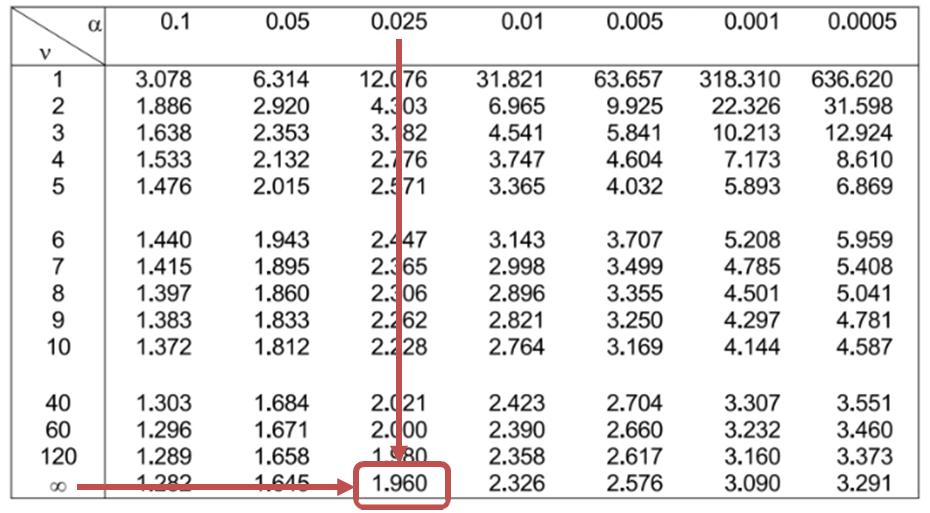
The degrees of freedom amount to \(n-1=2,050-1=2,049\); thus, the critical values are \(\pm 1.960\). Therefore, we will reject the null hypothesis if the calculated t-statistic is less than -1.96 or greater than 1.96.

Step 5: Calculate the test statistic:

Note that from the table \(\bar{d}=-0.0022\) and \(s_d=0.3321\) so that the t-statistic is given:

$$ t=\frac {\bar d-\mu_{d0}}{s_{\bar d}} =\frac {-0.0022-0}{\frac {0.3321}{\sqrt{2050}}}=-0.30 $$

Step 6: Make a Decision:

-0.30 falls within the bounds of the critical values of \(\pm 1.960\). As such, there is insufficient evidence to show that the mean of the differences in returns differs from zero.

Test Variance and Equality of Variance

Testing of a Single Variance

A chi-square test helps determine if a hypothesized variance value matches the true population variance. Unlike other distributions in the CFA® Program, the chi-square distribution is asymmetrical. Yet, as degrees of freedom increase, it approaches a more normal distribution.

As a natural consequence, the chi-square distribution has no negative values and is bounded by zero. A chi-square statistic with \((n – 1)\) degrees of freedom is computed as:

$$ { \chi }_{ n-1 }^{ 2 }=\frac { \left( n-1 \right) { S }^{ 2 } }{ { \sigma }_{ 0 }^{ 2 } } $$

Where:

\(n\) = Sample size.

\(S^2\) = Sample variance.

\({ \sigma }_{ 0 }^{ 2 }\) = Hypothesized population variance.

Example: Chi-square Test

For the 15-year period between 1995 and 2010, ABC’s monthly return had a standard deviation of 5%. John Matthew, CFA, wishes to establish whether the standard deviation witnessed during that period still adequately describes the long-term standard deviation of the company’s return. To achieve this end, he collects data on the monthly returns recorded between January 1, 2015, and December 31, 2016, and computes a monthly standard deviation of 4%.

Carry out a 5% test to determine if the standard deviation computed in the latter period differs from the 15-year value.

Solution

As is the norm, start by writing down the hypothesis.

\(H_0: \sigma_0^2= 0.0025\)

\(H_1: \sigma^2 \neq 0.0025\)

Since the latter period has 24 months, \(n = 24\), the test statistic is:

$$ { \chi }_{ 24-1 }^{ 2 }=\frac { \left( 24-1 \right) { 0.0016 } }{ 0.0025 } =14.72 $$

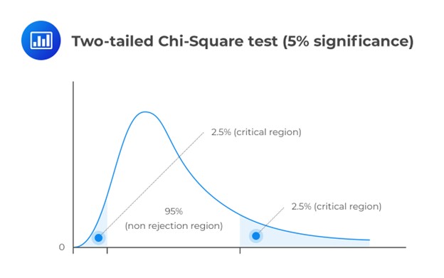
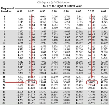
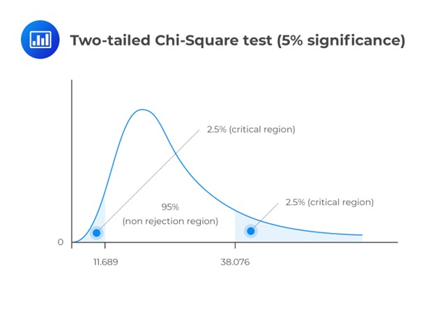
This is a two-tailed test. As such, we have to divide the significance level by two and screen our test statistic against the lower and upper 2.5% points of \({ \chi }_{ 23 }^{ 2 }\).

Consulting the chi-square table, the test statistic (14.72) lies between the lower (11.689) and the upper (38.076) 2.5% points of the chi-square distribution.

Note that you will be given a simplified critical value table in the exam situation.

Evidently, we have insufficient evidence to reject the \(H_0\). It is, therefore, reasonable to conclude that the latter standard deviation value is close enough to the 15-year value.

Test Concerning the Equality of the Variances

To test the equality concerning the variances, we use the F-test. Assume that we have 2 independent random samples of sizes n1 and n2 from \(N(\mu_1, \sigma_1^2)\) and \(N(\mu_2, \sigma_2^2)\).

Also, let us consider a scenario where we have the sample variances as \(S_1^2\) and \(S_2^2\). The basic situation usually involves the following hypothesis:

\(H_0: \sigma_1^2 =\sigma_2^2\)

\(H_a: \sigma_1^2 \neq \sigma_2^2\)

The test statistic is \(\frac {S_1^2}{S_2^2} \sim F_{n1 – 1, n2 – 1 } \text{ under } H_0\).

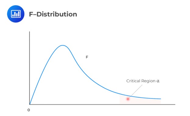
The decision rule is to reject the null hypothesis if the test statistic falls within the critical region of the F-distribution.

Example: F-test

An analyst is studying whether the population variance of returns on a commodity index changed after the introduction of new trading guidelines. The first 320 weeks elapsed before the guidelines were introduced, and the second 320 weeks came after the introduction. The analyst gathers the data in the table below for 320 weeks of returns before and after the change in guidelines.

$$ \begin{array}{c|c|c}
& \textbf{Mean Weekly} & {\textbf{Variance of}} \\
& \textbf{Return (%)} & \textbf{Returns} \\ \hline
\text{Before guidelines change} & 0.180 & 3.520 \\ \hline
\text{After guidelines change} & 0.090 & 2.967
\end{array} $$

Do the variances of returns differ before and after the guideline change? Employ a 5 percent significance level.

Solution

Step 1: State the hypothesis:

$$ H_0:\sigma_{\text{Before}}^2=\sigma_{\text{After}}^2 \text{ vs } H_a:\sigma_{\text{Before}}^2\neq\sigma_{\text{After}}^2 $$

Step 2: Identify the appropriate t-statistic:

$$ t=\frac{s_{\text{Before}}^2}{s_{\text{After}}^2} $$

Step 3: Specify the level of significance:

$$ \alpha = 5\% \text{ (two-tailed)} $$

Step 4: State the decision rule:

$$ \begin{align*} \text{Left side} & = 0.803 \\
\text{Right side} & = 1.246 \end{align*} $$

Reject the null if the calculated t-statistic is less than 0.803 and reject the null if the calculated t-statistic is greater than 1.246.

Step 5: Calculate the test statistic:

$$ t=\frac{s_{\text{Before}}^2}{s_{\text{After}}^2}=\frac{3.520}{2.967}=1.1864 $$

Step 6: Make a decision:

Fail to reject the null hypothesis because 1.1864 falls within the bounds of the critical values of [0.80,1.246]. There is insufficient evidence to indicate that the weekly variances of returns are different in the periods before and after the guidelines change.