Present Values, Future Values, Annuiti ...
Future Values The Future Value (FV) of a Single Sum of Cash Flow... Read More
The classic normal linear regression model assumptions are as follows:
I. The relationship between the dependent variable, Y, and the independent variable, X, is linear.
A linear relationship implies that the change in Y due to a one unit change in X is constant, regardless of the value taken by X. If the relationship between the two is not linear, the regression model will not capture the trend accurattely, a situation that will result in inaccurate predictions. The model will be biased and either underestimate or overestimate Y at various points. For example, the model \(Y = \beta_{0}+\beta_{1}e^{\beta_{1}x}\) is non linear in \(β_{1}\), and therefore we should not attempt to fit a linear model between X and Y.
It also follows that the independent variable, X, must be non stochastic (must not be random). A random independent variable rules out a linear relationship between the dependent and independent variables.
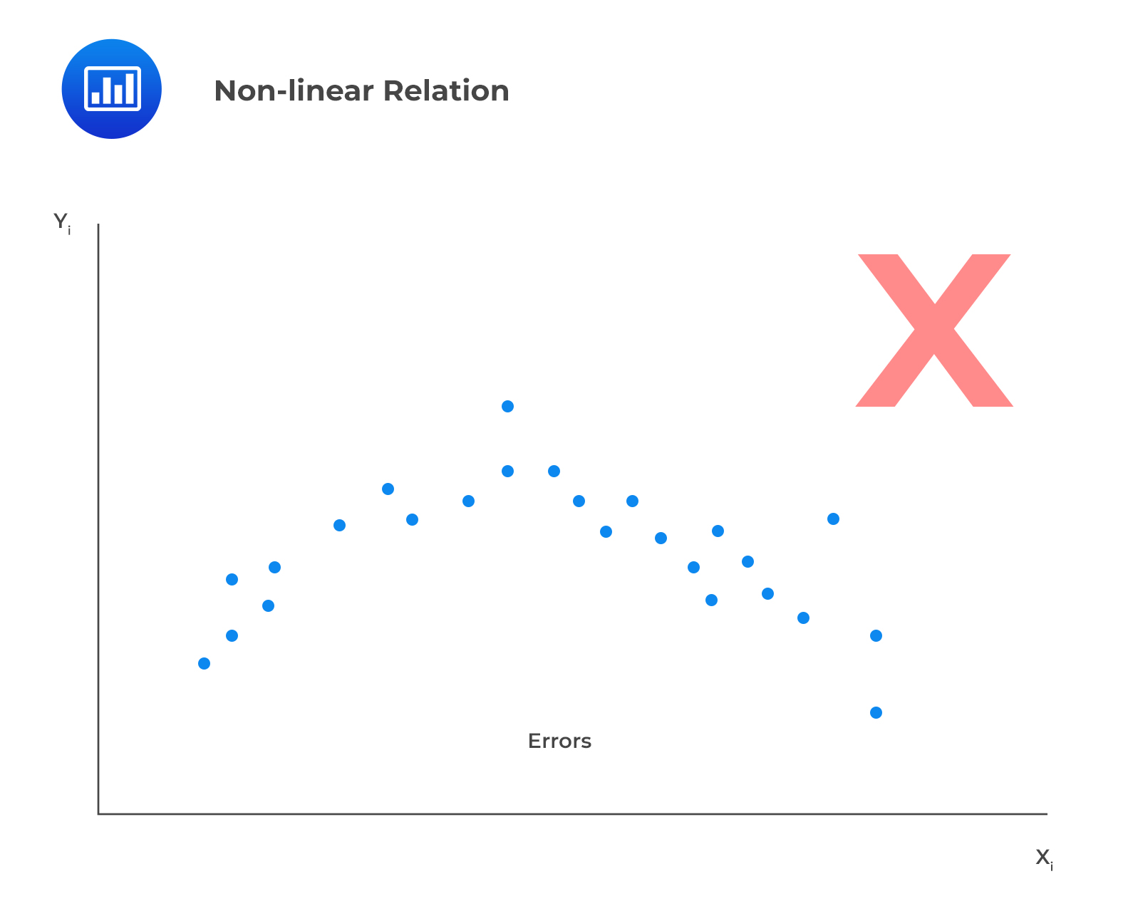
In addition, linearity means the residuals should not exhibit a discernible pattern when plotted against the independent variable but should instead be completely random. In the example below, we’re looking at a scenario where the residuals appear to show a pattern when plotted against the independent variable, X. This effectively serves as evidence of a non-linear relation.

II. The expectation of the error terms is zero.
$$E(\epsilon)=0$$
III. The error terms (residuals) must be normally distributed.
A histogram of the residuals can be used to detect if the error term is normally distributed. A symmetric bell-shaped histogram indicates that the normality assumption is likely to be true.
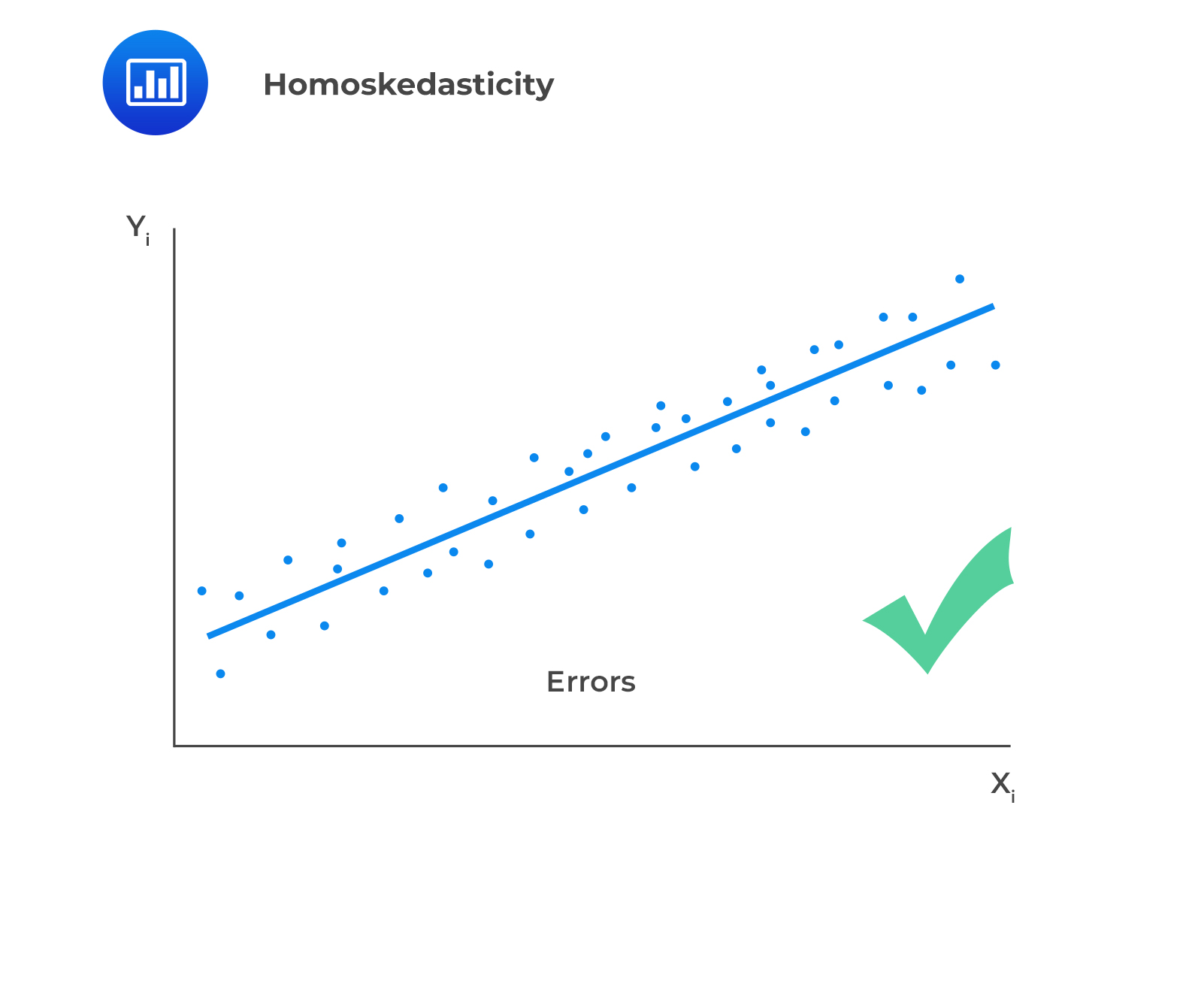
IV. The variance of the error terms is constant across all observations.
$$E(\epsilon_i^2)=\sigma_{\epsilon}^2,\ i=1,2, …, n$$
This assumption is also known as the homoskedasticity assumption.

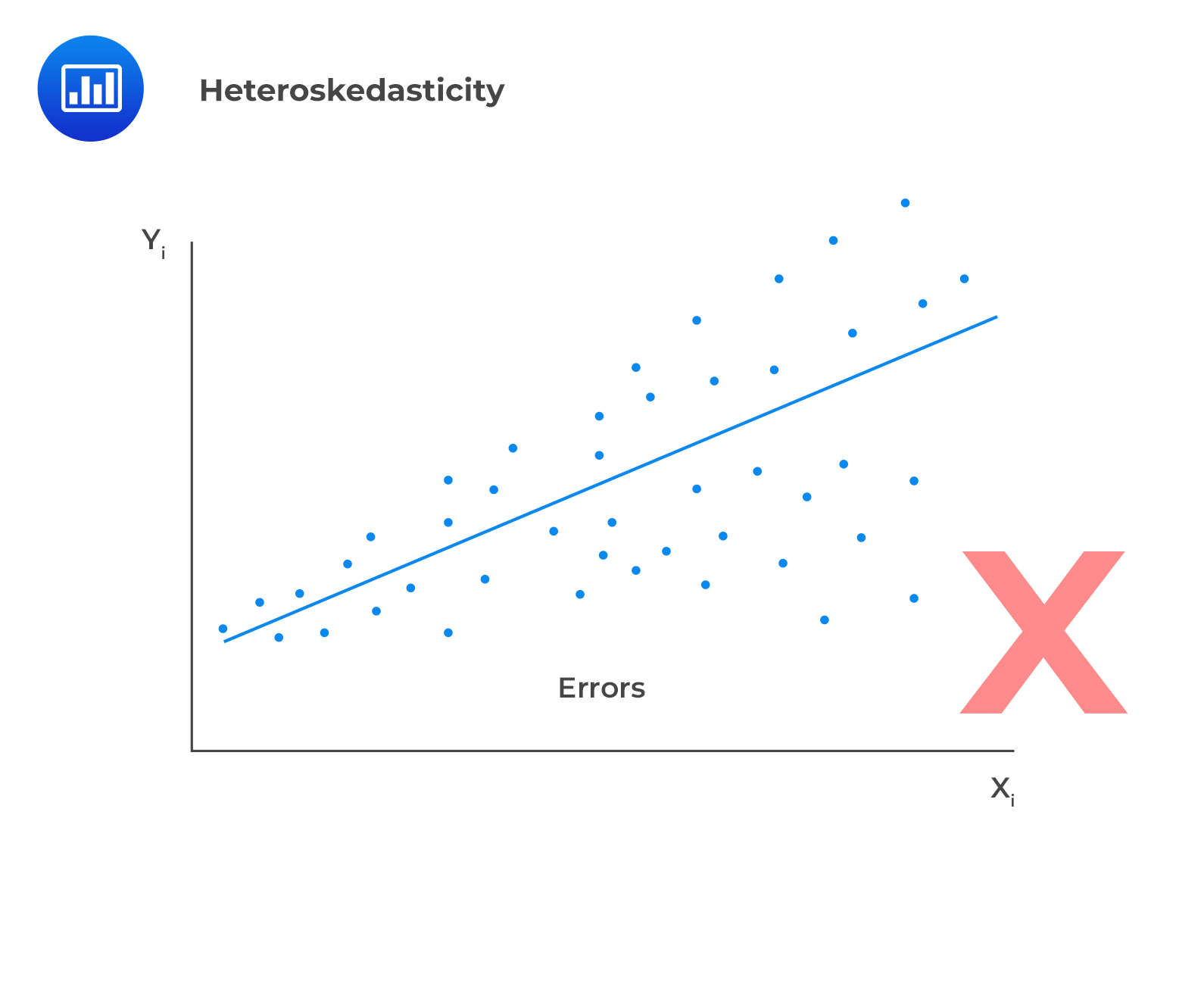
In case residuals and the predicted values increase simultaneously, then such a situation is known as heteroscedasticity (or heteroskedasticity).

To test for heteroscedasticity, one ought to plot the least square residuals against the independent variable. If there is an evident pattern in the plot, then that is a manifestation of heteroskedasticity.
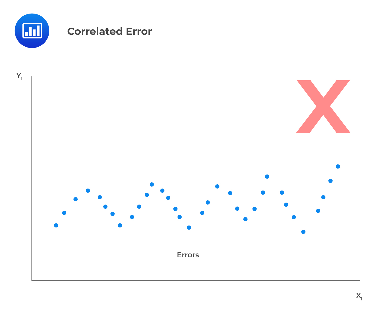
V. The error terms, \(\epsilon\), must be uncorrelated across all observations.
$$E(\epsilon_i\epsilon_j)=0,\ \forall i\neq j$$
To verify this assumption, one should use a residual time series plot, which is a plot of residuals versus time. Fluctuating patterns around zero will indicate that the error term is dependent.

Get Ahead on Your Study Prep This Cyber Monday! Save 35% on all CFA® and FRM® Unlimited Packages. Use code CYBERMONDAY at checkout. Offer ends Dec 1st.