Portfolio Management – Level I CFA® Program Essential Review Summary offered by AnaystPrep

Reading 51 – Portfolio Management: An Overview

Portfolio management is about creating a diversified approach to meet one’s investment goals. Diversification involves avoiding too much exposure to a single asset or asset type. Diversifying the risks of a portfolio helps reduce downside risk without necessarily decreasing the expected rate of return. Portfolio risk is measured by the standard deviation of returns, and the correlations between different assets can lead to decreased overall risk when combined. The principle behind this diversification effect is based on Harry Markowitz’s research and is known as Modern Portfolio Theory.

There are two broad categories of investors: individuals and institutions. Individual Investors are individual people or families that are investing to meet their personal goals. Institutional Investors are professional organizations that represent a variety of investment goals. These include groups such as pension funds, endowments, banks, investments funds, and even charities.

Employees of public and private companies have retirement savings managed in accounts that can be either defined benefit or defined contribution. Defined Contribution plans involve employers making specific contributions to accounts that will accrue in value for their employees. The final amounts available for retirement will depend on the performance of financial markets. In a Defined Benefit plan, however, the employer is responsible for providing a set amount of financial benefits to their employees in retirement. This financial obligation means that the portfolio risk must be managed much more closely by the employer.

There is a series of steps that must be followed in the portfolio management process.

1. The Planning Step

The client’s investment objectives, constraints, and portfolio benchmark need to be documented in an Investment Policy Statement (IPS), which is the document by which the investments will be managed.

2. The Execution Step

a. Asset Allocation: The portfolio manager needs to develop a view on the risk and return expectations of various asset classes. This analysis step can be top-down (starting from high-level macroeconomic factors) or bottom-up (starting from company-specific information). Decisions are made as to the optimal allocation of the portfolio assets among available asset classes.

b. Security Analysis: Specific securities are chosen for purchase that fit into the asset classes chosen in the previous step.

c. Portfolio Construction: The information from the previous steps is used to create an investment portfolio. Securities are purchased and trades are executed.

3. The Feedback Step

The portfolio is monitored and rebalanced periodically to keep its exposures in line with the Investment Policy Statement. Performance is also tracked and reported to the client at regular intervals.

Asset managers can either be Active or Passive. Active asset managers attempt to outperform benchmarks through fundamental and quantitative research. Passive managers simply try to replicate the returns of a market index.

There can also be either Traditional or Alternative managers. Traditional managers focus on creating diversified portfolios for their clients by using long stocks and bonds. Alternative asset managers use leverages, derivatives, etc. to create a return that is uncorrelated to the market/to outperform a pre-determined index.

In addition to building a portfolio of specific investment assets, there are also pooled investment vehicles that can be purchased. Mutual Funds are one example, where each investor in the mutual fund owns a pro-rata claim on the value of the securities that the mutual fund owns. In an Open-End Fund, investors can buy or sell positions in the fund and the portfolio manager will adjust the holdings of the fund to meet these changes in investable assets. Closed-End Funds, on the other hand, do not create new shares to allow for investors to enter or exit the fund. There are a fixed number of shares in the fund and any new investor that wishes to purchase must buy existing shares from a current owner.

Funds can be classified as Load or No-Load funds depending on whether there is a fee that must be paid to buy or sell shares of the fund. No-Load funds typically charge an annual management fee that is a percentage of total fund assets.

Mutual funds are categorized by the assets in which they invest. Money Market Funds invest in very short-term debt and are often treated as a substitute for bank deposits. Bond Mutual Funds buy fixed income securities of varying maturities. Stock Mutual Funds buy equity securities and Hybrid/Balanced Funds buy combinations of different asset classes. Funds can be managed either actively or passively, with passive funds trying to closely match a given index through a buy-and-hold approach and active funds doing more buying and selling to try and maximize performance results.

Other types of pooled investment vehicles include Exchange Traded Funds (ETFs), which are similar to mutual funds except that shares trade on the open market. A new investor in a mutual fund buys shares at the end of day Net Asset Value directly from the mutual fund provider, while a new investor in an ETF buys shares on the exchange like they would do for a regular stock. Separately Managed Accounts are similar to mutual funds but are created specifically for an individual or institutional client. They can be customized to fit any manner of investment or tax strategy. Hedge Funds are typically more complex in nature and are more loosely regulated than mutual funds. They usually require high minimum investments and have liquidity restrictions on invested assets.

Reading 52 – Portfolio Risk and Return: Part I

The purpose of investing is to earn a return on your assets, so it’s important to be able to calculate that return and the risk taken on to achieve it. There are a number of different types of returns included in the curriculum. The simplest to calculate is the Holding Period Return. This is simply the total investment gains as a percentage of the starting amount:

$$ Return=\frac { Ending\quad Value-Starting\quad Value+Dividends }{ Starting\quad Value } $$

This will give you the return for a single holding period, but you will also need to know how to combine multiple return periods. The first of these combination methods is to calculate the Arithmetic Mean:

$$ Arithmetic\quad Mean\left( 5\%,10\%,15\% \right) =\frac { 5+10+15 }{ 3 } =10\% $$

A more complex approach to combining multiple return periods is the Geometric Mean. This utilizes the principle of compounding, so it’s more accurate as a method of calculating the returns of a portfolio over time. Remember to convert all percentages to decimal values when calculating the geometric mean

$$ Geometric\quad Mean\left( 5\%,10\%,15\% \right) =\left[ { \left( \left( 1+0.05 \right) \ast \left( 1+0.1 \right) \ast \left( 1+0.15 \right) \right) }^{ \frac { 1 }{ 3 } } \right] -1=9.9\% $$

One limitation of the arithmetic and geometric means is that they do not take into account the money invested in the portfolio over time. For example, if a portfolio experiences large growth early when its asset base is low and then lower returns in later years after attracting large new cash flows, its performance will look much better than what is experienced by most of the investors who were not around for the earliest years. The performance “per dollar” in the fund will be much lower than what the calculated means would indicate. Money-Weighted Returns take into account these flows by using the fund in- or out-flows to create a weighted average return. The IRR of a fund can also be useful in this regard. Similar to how it was used in the Quantitative Methods section, the Internal Rate of Return is the discount rate that sets the present value of the cumulative cash flows to zero.

The Money-Weighted Rate of Return (MWRR) is the IRR of a portfolio. It is the discount rate at which . You solve an MWRR problem the same way that you solve other IRR problems using your calculator. Since this method involves finding the PV of each cash flow, it is sensitive to when funds are invested or removed from the portfolio.

On the other hand, the Time Weighted Rate of Return (TWRR) is the geometric mean for a series of Holding Period Returns (HPRs).

$$ TWRR\quad of\quad a\quad portfolioformula =\left\{\left(1+{HPR}_1\right)^\ast\left(1+{HPR}_2\right)\ldots^\ast\left(1+{HPR}_n\right)\right\}-1 $$

By combining each holding period return into a geometric mean, the TWRR method gives a more robust return figure that is not influenced by the timing of cash flows.

You will sometimes need to compare returns for time periods of varying lengths. The Annualized Return calculation is used. Annualizing a return essentially compounds it by the number of times it takes for that period to equal one year. For example, to annualize a monthly return, you would compound it 12 times:

$$ Annualized\quad 5\%\quad monthly\quad Return={ \left( 1+0.05 \right) }^{ 12 }-1=79.6\% $$

Another important measure is the Portfolio Return, which is a weighted average return of all the components in a portfolio. Questions around this calculation typically give you the portfolio components and ask you to calculate the total return. All you do is multiply each component by its weight in the portfolio and add up the results.

All of the returns discussed so far do not factor in adjustments that must often be made when dealing with real investments and portfolios. You may be asked to calculate returns either Gross or Net of fees. Net returns are after all fees have been subtracted. Taxes are also relevant to most investments. Post-tax returns are what is left after taxes have been paid. The effects of inflation also impact investor returns. Nominal returns are what we have been calculating so far, and Real returns are when the effects of inflation are accounted for.

It’s important to understand the relative risk and return characteristics of major asset classes. For US equity securities, the smaller the company is, the higher the average return and variance of returns are. In fixed income securities, the longer the maturity of the security, the higher the average return (yield) and variance of return. Corporate bonds also return more (with higher variance) than government bonds of the same maturity. The primary concept to grasp when looking at the risk and return characteristics of different asset classes is that a higher average return with higher variance means that you can not expect to get that increased performance consistently. A higher variance means you will see wide fluctuations in returns between different years. The primary measurement of the variation of returns is in standard deviations, which are the square root of variance.

Return characteristics between asset classes utilize what is known as their variance/covariance relationships. These are based on a set of common data points that should look familiar from the Quantitative Methods section. Each asset class will have its own Mean returns, which refers to the average values they have over time. They will also have their own distinct Variance, which is the dispersion around the mean (basically the “risk” part of the risk/return framework). The Covariance of asset classes measures how closely they move in relation to one another. Assets that move very differently provide diversification benefits to the portfolio when added together.

Each investor will differ in how they view risk as part of their investment portfolio. Risk-Seeking behavior is when investors are willing to take on additional risk, even if it doesn’t seem like they are being adequately compensated for it with higher expected returns. Risk-Neutral investors will take on additional risk only when it’s accompanied by an appropriately higher return. Risk-Averse investors will avoid additional risk and accept lower returns as a result. This measurement of willingness to take on risk is known as Risk Tolerance.

Earlier we covered the simple calculation for the portfolio return, where you multiple each portfolio component’s return by its weight and then add these up. When it comes to risk in the portfolio, the calculation is a bit more complex (and you should know it, because you will probably get a question on this in your CFA level 1 exam). To calculate the standard deviation of a 2-asset portfolio, the formula is as follows:

$$ Portfolio\quad variance=\left( { w }_{ A }^{ 2 }\ast { \sigma }_{ A }^{ 2 } \right) +\left( { w }_{ B }^{ 2 }\ast { \sigma }_{ B }^{ 2 } \right) +\left( 2\ast { w }_{ A }\ast { w }_{ B }\ast { \sigma }_{ A }\ast { \sigma }_{ B }\ast { \rho }_{ AB } \right) $$
$$ w=portfolio\quad weight $$
$$ \sigma =standard\quad deviation $$
$$ \rho =correlation\quad coefficient $$
$$ Note:{ \sigma }_{ A }\ast { \sigma }_{ B }\ast { \rho }_{ AB }={ covariance }_{ AB } $$

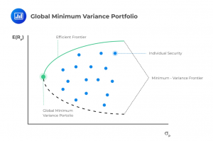
Since there is an infinite number of portfolios you could build based on different weights of asset classes, we need a way to determine what characteristics a portfolio needs to have to meet the needs of a specific investor. The Minimum-Variance Frontier is a way to model different portfolios along an axis of risk and return in order to find the most appropriate one. By choosing the portfolio with the least risk that meets the necessary return requirements, we ensure that an investor is maximizing their chances of meeting their investment goals. The line on the risk/return graph above which all portfolios meet the needed investment returns without undue risk is known as the Efficient Frontier, and is represented on the graph below.

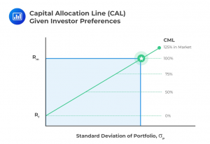
Another concept in this reading is known as the Capital Allocation Line (CAL), represented on the graph above. This is based on the principle of the two-fund separation theorem, which posits that all investors will hold a portfolio that combines two assets, one risk-free portfolio and one portfolio of risky assets. Breaking the portfolio into these components allows us to graph a line showing the expected risk and returns as the portfolio weight of the two assets changes. The line represented by this is the CAL. The investor’s optimal portfolio will appear along this line.

In order to determine the appropriate level of risk, it is necessary to calculate the investor’s Risk Aversion. The formula for this is:

$$ u=E\left( r \right) -\frac { 1 }{ 2 } A{ \sigma }^{ 2 } $$
$$ U=utility $$
$$ E\left( r \right)=expected\quad return $$
$$ A=risk\quad aversion\quad coefficient $$
$$ { \sigma }^{ 2 }=portfolio\quad variance $$
The risk aversion coefficient will be positive for risk-averse investors, zero for those risk neutral, and negative for those who are risk-seeking.

Reading 53 – Portfolio Risk and Return: Part II

As discussed in the previous reading, an investor’s risk tolerance can be quantified in portfolio construction using two assets: one totally risk-free and one composed of risky securities. The approach an investor takes can be determined by their level of risk tolerance and belief that they can achieve superior returns to the market. Investors that are more risk-averse and believe that they can only hope to match market returns will take a Passive investing approach, whereas more risk-tolerant investors who believe they can identify mispricings to outperform the market will take an Active investing approach.

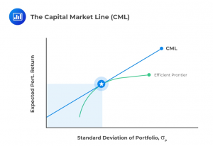
This principle leads to the use of the Capital Market Line (CML). This is a case of the Capital Allocation Line (CAL), where the risky asset in the equation represents the entire market portfolio. We use this approach to find the most appropriate portfolio by looking at where on a graph the risk/return line for the portfolio matches up to the efficient frontier (which is covered in the previous section as well).

The return and variance for the portfolio found using this method is calculated as:

$$ { R }_{ p }=w{ R }_{ f }+\left( 1-w \right) { R }_{ m } $$
$$ { \sigma }_{ p }^{ 2 }={ \left( 1-w \right) }^{ 2 }{ \sigma }_{ m }^{ 2 } $$
$$ { R }_{ f }=risk\quad free\quad return $$
$$ { R }_{ m }=market\quad return $$
$$ { \sigma }_{ p }=portfolio\quad std\quad dev $$
$$ { \sigma }_{ m }=market\quad std\quad dev $$

The risk an investor takes on by buying risky assets can be broken down into two categories: Systematic and Non-Systematic. Systematic Risk is the risk inherent to investment markets in general. It reflects the impacts of things like the business cycle or political uncertainty. This risk cannot be diversified away. Non-Systematic Risk is the risk inherent to specific assets or asset classes. It can be diversified away by purchasing assets with low or negative correlations. Investors should try to avoid (or diversify away if possible) any risk for which they are not compensated by higher returns.

The curriculum describes several models that investors can use to estimate the return of a portfolio based on the assets they plan to include. The most common type of these is a Multi-Factor Model, which allows for several inputs in order to model the expected return. These models can use macroeconomic, statistical, or fundamental factors that can be combined in order to develop the most appropriate estimate of expected return. A common calculation approach is to find a sum of the return attributed to each return factor multiplied by their respective Betas. This “weighted average” result will approximate the expected return based on the historical returns and the exposure to/correlation with the investment portfolio.

One of the most common multi-factor models is the three-factor model developed by Fama and French, which was later expanded to four factors. The original three factors they included were relative size of the company, relative book-to-market value of the company, and the market beta. The fourth factor added later was security momentum.

The simplest type of return generating model is the single factor model. A common model of this type is the emarket model, where returns are estimated based on the exposure to the market:

$$ R={ R }_{ f }\left( 1-\beta \right) +\beta { R }_{ m } $$
$$ { R }_{ f }=risk\quad free\quad rate $$
$$ { R }_{ m }=market\quad return $$
$$ \beta =market\quad beta $$

Multi-factor models build on this concept by including more factors and their respective betas in order to break down the components of the expected return.

Calculating the risk of these portfolios (the exam typically will most likely ask for risk calculations for single-factor models due to the complexity of multi-factor formulas) is similar to other multiple asset portfolios but simplified slightly because the risk (and therefore correlation) of the risk-free asset is zero. As a result, the calculated Beta for a single factor portfolio is:

$$ \beta =\frac { Covariance\left( { R }_{ p },{ R }_{ m } \right) }{ { \sigma }_{ m } } $$

Interpreting beta is the same as correlation was used in the Quantitative Methods section. A positive market beta means the asset moves in the same direction as the market, while a negative value means they move differently. Unlike correlation, beta values can be more than 1 and less than -1.

The Capital Asset Pricing Model (CAPM) is used to illustrate a linear relationship between the expected return and risk of an investment asset. Since it is is a simplified view, it relies on a series of assumptions about market behaviors that will not always line up with real-world results. The primary assumptions of the model include that all investors are risk-averse, utility-maximizing, and fully rational. This assumption is necessary to make the model behavior more predictable, but it’s important to remember that investors in real life exhibit a wide variety of behaviors based on their own risk tolerance and preferences. The CAPM also assumes that there are no transactions costs or taxes and that investments are only held for one, uniform-length holding period.

The Security Market Line (SML) is the graphical representation of the CAPM using beta as the x-axis and expected return on the y-axis. The SML can be represented formulaically as:

$$ E\left( { R }_{ p } \right) ={ R }_{ f }+\beta \left( E\left( { R }_{ m } \right) -{ R }_{ f } \right) $$

In this formula, the expected return of the portfolio is the risk-free rate plus the risk premium (market return minus risk-free rate) times the market beta. This is a crucial concept for your CFA level 1 exam.

The returns calculated using the CAPM and other models can be used in a number of ways related to portfolio management. The data they provide serve as inputs for several important formulas that show up repeatedly on the exam, and also on the level 2 and 3 exams. The Sharpe Ratio is the slope of the CAL and is calculated as the risk premium divided by the standard deviation of the portfolio. It tells you how much return you are getting in exchange for taking on additional risk. The Treynor Ratio is similar to the Sharpe ratio but uses the market beta as the dividend. It tells you how much additional risk you are taking on relative to total risk. The M-squared Ratio tells you the weight of the risky asset you want in the portfolio in order to set portfolio risk equal to market risk. Jensen’s Alpha finds the difference between the actual return of the portfolio and the calculated, risk-adjusted return.

$$ Sharpe\quad Ratio=\frac { { R }_{ p }-{ R }_{ f } }{ { \sigma }_{ p } } $$
$$ Treynor\quad Ratio=\frac { { R }_{ p }-{ R }_{ f } }{ { \beta }_{ p } } $$
$$ M-squared\quad { w }_{ p }=\frac { { \sigma }_{ m } }{ { \sigma }_{ p } } $$
$$ Jensen’s\quad alpha={ R }_{ p }-\left[ { R }_{ f }+{ \beta }_{ p }\left( { R }_{ m }-{ R }_{ f } \right) \right] $$

FRM Part I & Part II Complete Course

Reading 54 – Basics of Portfolio Planning and Construction

The most important part of constructing an investment portfolio is making sure that you have a solid understanding of the investment objectives that you are trying to achieve. The document that captures all of the appropriate investment goals and constraints is known as the Investment Policy Statement (IPS). As outlined in the curriculum (and in the curriculum for future levels), the creation of the IPS is the first part of an advisor’s job when working to determine the best approach for a client.

A typical IPS will follow the structure below:

• Introduction
  • Description of the client
• Statement of Purpose
  • Purpose of the IPS
• Statement of Duties and Responsibilities
  • Duties and responsibilities of all parties – client, advisor, custodians, etc.
• Procedures
  • The steps that will be undertaken to keep the IPS updated and procedures to respond to various contingencies
• Investment Objectives
  • The client’s investment objectives
• Investment Constraints
  • The client’s investment constraints
• Investment Guidelines
  • Information on how the investment policy should be executed and includes the permissibility and exclusion of assets
• Evaluation and Review
  • Guidance on obtaining feedback for investment results
• Appendices
  • Strategic Asset Allocation; the policy portfolio that provides the baseline portfolio asset allocation
  • Rebalancing policy

The primary components of the IPS that relate to the portfolio construction process are the investment objectives and constraints. These will outline the return and risk guidelines that will need to be followed throughout the portfolio creation and management process. The client’s risk objectives must be clearly defined and can be stated in either absolute or relative terms. Their risk tolerance is a function of both their willingness and ability to bear risk and needs to reflect both concerns. Willingness represents the client’s psychological comfort with investment risk, while Ability is a quantitative measure of the client’s assets and financial ability to absorb losses and volatility. When the willingness and ability are not in alignment, it is up to the advisor to explain the implications of this to the client even though it is often not possible to change the client’s mind. The prudent action is to adhere to the risk tolerance that is the lower of the two factors.

Similarly, the return objectives can be defined in either absolute or relative terms. These are typically based on an appropriate benchmark measure. For cases like a pension fund, the return objectives can be based on specific obligations that the portfolio is responsible for meeting. These returns should be stated as gross or net of fees and taxes and need to be appropriate based on the conditions of the broader market and macroeconomic factors.

There are several important investment constraints that must be outlined in the IPS that will impact how the portfolio is constructed and managed. Liquidity needs must be specified if they can be quantified and, if they cannot be, accounted for to create certainty that future cash flow needs can reasonably be met. The investment Time Horizon is an important concern that will affect which assets or asset classes can be included in the portfolio. Tax Concerns have a tremendous effect on investment results and so much be properly accounted for by the advisor. Legal and Regulatory Factors are more varied by where the client and the portfolio reside and will sometimes involve the use of outside experts such as lawyers to handle properly. Unique Circumstances is the final major category of limitation and covers any special concerns that do not fit in the previous sections. These concerns are often referred to as “ESG”, which stands for Environmental, Social, and Governance. This section includes numerous ethical, religious, or other limitations on how the client can invest their money.

The first step in building a portfolio according to the information in the IPS is making the asset allocation decisions. The primary predictor of long-term returns is the asset allocation of the portfolio. The Strategic Asset Allocation (SAA) is the formal specification for how portfolio funds will be invested among available asset classes. The Capital Market Expectations for each asset class will determine the expected performance of the portfolio once it is allocated among available investment options. The level of granularity among asset classes used to specify the SAA is somewhat flexible according to client preferences. How broadly or narrowly they define each asset class is up to them as long as they adhere to a few criteria. The risk and return characteristics must be homogeneous among assets within each class, each class must be mutually exclusive, and each class must be a representation of the investable universe.
Environmental, Social and Governance (ESG) considerations can be implemented across all asset classes. Investors may choose to not invest in asset classes that go against ESG considerations, for example, by instructing the asset manager not to invest in military equipment stocks. There are some benchmarks that reflect excluded companies and sectors.

Reading 55 – Risk Management: An Introduction

Risk management is an important part of managing an investment portfolio. At an institutional level, risk management can include risks to the financial investments as well as operational risks on the enterprise side. For individuals, risk management is often more informal and unstructured.

A proper risk management framework is necessary for an institution to properly track and manage risks to its investment outcomes, regardless of the sources of risk. There are a number of important areas to be addressed by this framework. Risk Governance is the top-level system of structures and policies that ensures risk management supports the entire enterprise. Risk Identification and Measurement is the quantitative tracking and monitoring risk exposures. Risk Infrastructure refers to the people and systems that carry out the risk management process. Policies and Processes provide constraints and guidelines for the ongoing daily operations of the firm. Risk Monitoring, Mitigation, and Management is the continuous evaluation of current and potential risk exposures. Communication is important to keep risk information available to all affected parties in the organization. Strategic Analysis or Integration analysis identifies which risk activities are improving the process outcomes and which ones can be removed.

Having a risk management framework will reduce the frequency of surprises that impact the investment outcomes of the firm. It also increases the discipline around decision making and reduces operational errors. The results of having a proper framework include reputational improvements and better relationships with regulating entities.

Effective risk governance involves a visible commitment from a firm’s governing body. They must be comfortable discussing risk exposures and taking preventative action even in periods of relative calm. This process needs to be comprehensive around the entire enterprise and include concerns for risks that cannot be captured through quantitative measures.

Any investor must identify the risk tolerance they have in order to set their investment expectations. There are many factors that go into this determination, including the ability to withstand losses, the competitive landscape, and the regulatory environment in which they do business. The risk tolerance should not reflect personal motivations or beliefs. The tolerance should be determined in a non-crisis period so that it can serve as a strategic guideline over a long period of time.

Risk budgeting is a strategy to set useful guidelines by which day-to-day investment decisions can be made. The risk budget will quantify risk and allocate the exposures across the organization. Common risk measures used for budgeting include Standard Deviation, Beta, Value at Risk, and Scenario Losses. Multi-dimensional approaches combine several factors in order to provide a more comprehensive view of risk.

Reading 56 – Technical Analysis

Technical analysis is the practice of using price and volume data to value stocks. There are a number of concepts you’ll be expected to understand related to technical analysis on the exam. One of these is Trend, which is a when a security consistently keeps moving upward or downward over time. This is the market’s way of reflecting a difference between supply and demand that can persist for a while.

Another important concept is that is Support and Resistance levels. These are price points where market activity tends to keep a security from going below (Support) or above (Resistance). These levels can act as floors or ceilings to the trading level of a security.

Related to the previous concept is that of the Change in Polarity. This is the principle that when a Support or Resistance level is breached, it then becomes its opposite. This can occur when a Resistance level is exceeded and that price point becomes a new Support for trading activity at the new higher level.

In the field of technical analysis, there are a number of patterns that appear on stock charts reflecting price movements that can be used when trying to forecast future movements in stock price. These chart patterns fall into a few categories. Reversal Patterns indicate that a trend is likely to reverse from the direction it has been going. A common example is the “Head and Shoulders” pattern that usually signals the end of an uptrend.

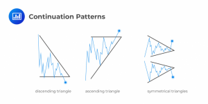
Another category of chart pattern is the Continuation Pattern. These patterns are used to identify trends that will continue after a pause. Many common continuation patterns are based on triangles that highlight trading movement that is converging to a given point in the future.

In addition to chart patterns, there are also indicators used in technical analysis that are used to predict future changes in a security’s price. The four categories of indicators are:

1. Price-Based Indicators

These indicators use information about the security’s past and current price to try and predict future prices. A simple example of this is the moving average, which is the average price of a security over a number of previous time periods. This average removes the oldest observation every time a new observation is added. Bollinger Bands are another common indicator based on price. These are lines that indicate the standard deviations of prices compared to a moving average of the stock’s price.

2. Momentum Oscillators

These are values calculated by finding the difference between the most recent price of a security and a previous price on a specified day in the past. Watching for the calculated value to switch from positive to negative is one indicator of a potential trend reversal

3. Sentiment Indicators

These are various polls that are conducted to gauge the sentiment of individual investors or investment professionals about the state of the equity market.

4. Flow-of-Funds Indicators

These measure the movement of money into and out of rising and declining stocks to identify upward or downward trending behavior. One of the most useful here is the Arms Index:

Values above 1 indicate more volume in declining stocks, while values below 1 indicate more activity in rising stocks.

Another category in the field of technical analysis used to forecast market price movements is Cycles. These are patterns of market movement that reoccur over various time frames. There are cycles that can happen multiple times throughout a trading day or take many years to complete one occurrence.

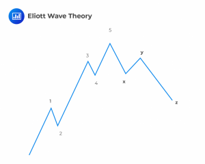
Related to the analysis of cycles is the Elliott Wave Theory, developed in the late 1930s. This theory posits that there are repetitive and predictable cycles that can be observed in stock price movements. The theory dictates that there is a pattern of cycles consisting of activity waves. A cycle will contain 5 waves moving in the direction of the main market trend and then 3 waves moving in the opposite direction. The size of each wave is related to the one preceding it based on the Fibonacci number sequence.

Reading 57 – Fintech in Investment Management

The word “Fintech” is simply a combination of the words “financial” and “technology.” Today, fintech encompasses more advanced systems that are able to analyze information and make decisions based on machine-learning logic. Machines that “learn” how to perform tasks over time have been developed. These systems can often surpass human capabilities.

Big data is a term used to refer to complex, extremely large data that may be analyzed computationally to reveal patterns, trends, and associations, especially those leading to human behavior. It encompasses both Traditional Data Sources such as company reports, stock exchange sources, and data gathered from governments as well as Nontraditional (Alternative) Data from social media, sensor networks, and electronic devices. Data can be Structured Data (organized in tables and are commonly stored in a database), Unstructured Data (cannot be presented in tabular forms, such as text messages, tweets, and emails) or Semi-structured Data (a mix of both).

Artificial Intelligence (AI) has much to do with the development of computer systems that exhibit cognitive and decision-making abilities comparable or superior to that of humans. Machine Learning is a current application of AI which revolves around the idea that we should really just give machines access to data and let them learn by themselves without further human intervention. Machine learning can take the form of Supervised Learning (supervised by humans) or Unsupervised Learning, where computers are only given input data and are tasked with describing the data, for instance by grouping or clustering of data points.

The ability to create computer programs that can learn on their own and improve over time creates new opportunities for investment professionals across the board, which include the Analysis of Loads of Data through complex algorithms developed to scour social media and sensor networks in search of consumer sentiments and product performance data that can be integrated into a manager’s buy/sell decisions, Automated Trading to identify systematic investment strategies and automatically execute multiple trades over several financial markets worldwide, Analytical Tools to identify systematic investment strategies and automatically execute multiple trades over several financial markets worldwide, and Automated Advice through robo-advisors.

Another application of fintech is the Distributed Ledger Technology (DLT). A distributed ledger is a database held and updated independently by each participant (or node) in a large network. Rather than have a central authority, records are independently constructed and held by every node (computer). DLT has several features that make it a favorite among investment managers. Cryptography refers to algorithmic encryption of data such that it is unusable in the hands of an unauthorized party. As a result, DLT has a high level of security and integrity. Smart Contracts are computer programs that self-execute on the basis of pre-specified terms and conditions. If a counterparty defaults on a payment, collateral can be transferred to the relevant party instantaneously. Blockchain is a type of digital ledger in which information, such as changes in ownership of an asset, is recorded sequentially within blocks that are then linked together and secured using cryptography.

The most common use of the distributed ledger technology (DLT) is Bitcoin, a Cryptocurrency which enables payments to be sent between users without passing through a central authority. Other uses include Tokenization (the process of converting rights to an asset), Post-trade Clearing and Settlement (near-real-time trade verification, reconciliation, and settlement) and Seamless Compliance, which would eliminate the need for large post-trade monitoring teams and create operational efficiency.

FRM Part I & Part II Complete Course