Evolution of Portfolio Theory Efficient Frontier to SML (Calculations for CFA® and FRM® Exams)

21 Dec 2020

Evolution of Portfolio Theory

In theory, we could form a portfolio made up of all investable assets, however, this is not practical and we must find a way of filtering the investable universe. A risk-averse investor wants to find the combination of portfolio assets that minimizes risk for a given level of return.

Minimum-variance Frontier

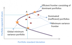
As we form a portfolio of assets, we can determine the portfolio return-risk characteristics that are a function of the characteristics of the underlying portfolio holdings and the correlation between the holdings. By varying the allocation to the underlying assets, we derive an investment opportunity set of different portfolio compositions. This is made up of the various combinations of risky assets that lead to specific portfolio risk-return characteristic which can be graphically plotted with portfolio expected return as the y-axis and portfolio standard deviation as the x-axis.

For each level of return, the portfolio with the minimum risk will be selected by a risk-averse investor. This minimization of risk for each level of return creates a minimum-variance frontier – a collection of all the minimum-variance (minimum-standard deviation) portfolios. At a point along this minimum-variance frontier curve, there exists a minimum-variance portfolio which produces the highest returns per unit of risk.

Global Minimum-variance Portfolio

Along the minimum-variance frontier, the left-most point is a portfolio with minimum variance when compared to all possible portfolios of risky assets. This is known as the global minimum-variance portfolio. An investor cannot hold a portfolio of risky (note: risk-free assets are excluded at this point) assets with a lower risk than the global minimum-variance portfolio.

Efficient Frontier

The portion of the minimum-variance curve that lies above and to the right of the global minimum variance portfolio is known as the Markowitz efficient frontier as it contains all portfolios that rational, risk-averse investors would choose. We can also monitor the slope of the efficient frontier, the change in units of return per units of risk. As we move to higher levels of risk, the resulting increase in return begins to diminish. The slope begins to flatten. This means we cannot achieve ever-increasing returns as we take on more risk, quite the opposite. Investors experience a diminishing increase in potential returns as portfolio risk is increased. The developments can be explained using the slope of the efficient frontier:

Example 1

Which statement best describes the global minimum-variance portfolio?

A. The global minimum variance portfolio gives investors the highest levels of returns

B. The global minimum variance portfolio gives investors the lowest risk portfolio made up of risky assets

C. The global minimum variance portfolio lies to the right of the efficient frontier

Solution

The correct answer is B.

The global minimum variance portfolio lies to the far left of the efficient frontier and is made up of the portfolio of risky assets that produces the minimum risk for an investor.

The Two-Fund Separation Theorem

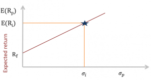
The two-fund separation theorem states that all investors regardless of taste, risk preference and initial wealth will hold a combination of two portfolios or funds: a risk-free asset and an optimal portfolio of risky assets. This allows us to break the portfolio construction problem into two distinct steps: an investment decision and a financing decision. Firstly, the optimal risky asset portfolio using the risk, return and correlation characteristics of the underlying assets dictate the investment decision. Secondly, considering an investor’s risk preference, a determination is made on the allocation to the risk-free asset. Plotting graphically the risk-free asset with the risky portfolio creates the capital allocation line (CAL).

Capital Allocation Line (CAL)

Capital allocation line (CAL) is a graph created by investors to measure the risk of a risk-free asset and risky asset (the risky asset represents multiple portfolios available to the investor). It is a line created on a graph of all possible combinations of risk-free and risky assets. Illustrated as follows:

Utility and Indifference Curves

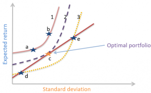
Utility is a measure of relative satisfaction that an investor derives from different portfolios. We can generate a mathematical function to represent this utility that is a function of the portfolio expected return, the portfolio variance and a measure of risk aversion.

$$U=E(r)-\frac{1}{2}A\sigma^2$$

Where:

$U$= utility

$E(r)$= portfolio expected return

$A$= risk aversion coefficient

$\sigma^2$= portfolio variance

In determining the risk aversion (A), we measure the marginal reward an investor needs in order to take on more risk. A risk-averse investor will need a high margin reward for taking on more risk. The utility equation shows the following:

Utility can be positive or negative – it is unbounded.
High returns add to utility.
High variance reduces utility.
Utility does not measure satisfaction but can be used to rank portfolios.

The risk aversion coefficient, A, is positive for risk-averse investors (any increase in risk reduces utility), it is 0 for risk-neutral investors (changes in risk do not affect utility) and negative for risk-seeking investors (additional risk increases utility).

To get the optimal portfolio, combine the indifference curves with the CAL:

The Market

The market includes all risky assets or anything that has value – stocks, bonds, real estate, human capital, commodities – these are all assets defined in “the market.” Not all market assets are tradeable or investable. If global assets are considered, there are hundreds of thousands of individual securities that make up the market that are considered tradable and investable. A typical investor is likely to be more concerned with their local or regional stock market as a measure of “the market”.

FRM Part I & Part II Complete Course

The Capital Market Line (CML)

The Capital Market Line (CML) is a special case of the CAL – the line which makes up the allocation between a risk-free asset and a risky portfolio for an investor. In the case of the CML, the risk portfolio is the market portfolio. Where an investor has defined “the market” to be their domestic stock market index, the expected return of the market is expressed as the expected return of that index. The risk-return characteristics for the potential risk asset portfolios can be plotted to generate a Markowitz efficient frontier. Where the line from the risk-free asset touches, or is tangential, to the Markowitz portfolio, this is defined as the market portfolio. The line connecting the risk-free asset with the market portfolio is the CML, illustrated in the graph below:

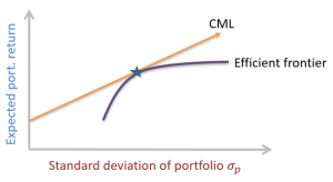
$$E(R_p)=R_f+\frac{E(R_m)-R_f}{\sigma_m}\times\sigma_p$$

This is the form of an equation of a straight line where the intercept is $R_f$ and the slope is $\frac{E(R_m)-R_f}{\sigma_m}$. This is the CML line which has a positive slope as the market return is greater than the risk-free return.

Security Market Line & CAPM

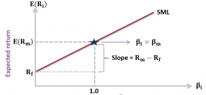
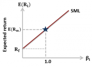
The Security Market Line (SML) is the graphical representation of the CAPM with beta reflecting systematic risk on the x-axis and expected return on the y-axis. The SML intersects the y-axis at the risk-free rate and the slope of the line is the market risk premium, $R_m-R_f$.