


Exam Study Tips for Postponed 2021 CFA ...
The CFA institute postponed the June exams and cancelled the December 2020 exams... Read More
The Time Value of Money is an important concept for the level 1 exam. You will need to be comfortable discounting the Present Value and Future Value of cash flows for individual and ongoing payments in the exam. Your calculator has functions built in to make these calculations easier. Here are the calculations that you need to know:
$$ FV=PV{ \left( 1+\frac { r }{ n } \right) }^{ n\ast t }
$$
$$ PV=\frac { FV }{ { \left( 1+\frac { r }{ n } \right) }^{ n\ast t } }
$$
$$ FV=Future\quad value $$
$$ PV=Present\quad Value $$
$$ r = discount \quad rate $$
$$ n = number \quad or\quad discounting\quad periods\quad per\quad year $$
$$ t = number\quad of\quad years $$
A simple example of this application is if you needed to determine how much you would pay today to receive $1 in one year, assuming your required rate of return was 5%. The formula would look like this:
$$ PV=\frac { $1 }{ \left( 1+.05 \right) } =$0.95 $$
Using this discount rate, $1 one year from now is worth $0.95 today.
You won’t often have to do the formulas written out by hand, but be familiar with them because the logic here applies to many other applications through this topic area. A similar issue that you’ll have to deal with involves ongoing cash flows such as annuities and perpetuities. Both involve finding the current value of a series of cash flows, just that an annuity continues for a certain period of time and a perpetuity never ends. The formulas for these are as follows:
$$ PV\quad Annuity=\frac { \left( 1-{ V }_{ n } \right) }{ r } $$
$$ r=rate\quad of\quad return $$
$$ n=term \quad of \quad annuity $$
$$ V={ \left( 1+r \right) }^{ -1 } $$
$$ PV\quad Annuity\quad Due=\frac { \left( 1-{ V }_{ n } \right) }{ d } $$
$$ d=\frac { r }{ \left( 1+r \right) } $$
$$ PV\quad Perpetuity=\frac { C }{ r } $$
$$ C\quad is\quad amount\quad of\quad each\quad payment $$
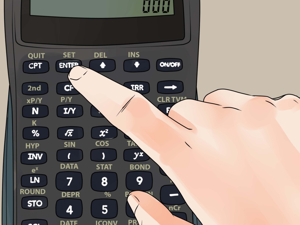
Your calculator has built-in functionality for PV and FV equations using the row of buttons labeled “N’, “I/Y”, “PV”, “PMT”, and “FV”. To use these for a problem, you input the value of all the parameters that you know and then have the calculator compute the missing value. To input a value, you type in the number for the value and then press the corresponding value’s button (i.e., to input 10,000 as the PV, you type in 10000, then press the “PV” button). Once you have input all figures you have, you press the CPT button and then the parameter button you want to calculate. Don’t forget to input the interest amount in decimals, so that 5% is entered as 0.05.
There are several methods of calculating the average value for a set of numbers as laid out in the curriculum. The formulas you need to know are:
$$ Arithmetic\quad Mean=\frac { \Sigma { X }_{ i } }{ N } $$
$$ Weighted\quad Mean=\sum _{ }^{ }{ { X }_{ i }{ W }_{ i } } $$
$$ Geometric\quad Mean={ \left( { X }_{ 1 }\ast { X }_{ 2 }\ast \dots \ast { X }_{ n } \right) }^{ \frac { 1 }{ n } } $$
$$ Harmonic\quad Mean=\frac { N }{ \sum _{ }^{ }{ \frac { 1 }{ { X }_{ i } } } } $$
$$ N=number\quad of\quad observations $$
$$ W=percentage\quad weight $$
Examples:
The Arithmetic Mean of the numbers \( { \left\{ 1,2,3,4 \right\} }\) is: \( \frac { 1+2+3+4 }{ 4 } =2.5\)
The Weighted Mean of a portfolio with the following assets is:
$$
\begin{array}
{} & Stocks & Bonds \\
Portfolio\quad Weight & 60\% & 40\% \\
Return & 10\% & 6\% \\
\end{array}
$$
$$ \left( 0.6\ast 0.1 \right) +\left( 0.4\ast 0.06 \right) =0.084 $$
The Geometric Mean of the numbers \( \left\{ { 1,2,3,4 } \right\} \) is:
$$ { \left( 1\ast 2\ast 3\ast 4 \right) }^{ \frac { 1 }{ 4 } }=2.21 $$
The Harmonic Mean of the numbers \( \left\{ { 1,2,3,4 } \right\} \) is:
$$ \frac { 4 }{ \frac { 1 }{ 1 } +\frac { 1 }{ 2 } +\frac { 1 }{ 3 } +\frac { 1 }{ 4 } } =1.92 $$
For the same set of numbers, it is always the case that:
Arithmetic Mean > Geometric Mean > Harmonic Mean
In addition to measures of average, there are several measurements of the distribution for datasets that you will need to know.
The Variance is the average of the squared deviations from the mean, and the formula to calculate this for a sample of data looks like this:
$$ { \sigma }^{ 2 }=\frac { \Sigma { \left( { X }_{ i }-\bar { X } \right) }^{ 2 } }{ n-1 } $$
$$ \bar { X }=Mean $$
The Standard Deviation is simply the square root of the variance.
The Mean Absolute Deviation is a measure of the average of the absolute values of deviations from the mean in a data set. We must use the absolute values because a sum of the deviations from the mean in a data set is always 0. This formula is as follows:
$$ MAD=\frac { \Sigma |{ X }_{ i }-\bar { X } | }{ n-1 } $$
Now we’ll calculate these values for the following returns data:
$$
\begin{array} \\
Year\quad 1 & Year\quad 2 & Year\quad 3 & Mean \\
10\% & 7\% & 5\% & 7.3\% \\
\end{array}
$$
$$ Variance={ \sigma }^{ 2 }=\frac { { \left( 0.1-0.073 \right) }^{ 2 }+{ \left( 0.07-0.073 \right) }^{ 2 }+{ \left( 0.05-0.073 \right) }^{ 2 } }{ 2 } =0.00063 $$
$$ Standard\quad Deviation={ \sigma }=\sqrt { 0.00063 } =0.025 $$
$$ MAD=\frac { |0.1-0.073|+|0.07-0.073|+|0.05-0.073| }{ 2 } =0.027 $$
Another important formula related to the previous metrics is the Sharpe Ratio. It measures the risk-adjusted returns of a portfolio. The higher the Sharpe Ratio of a portfolio, the more excess return you are getting for each additional unit of risk. This formula shows up repeatedly in all levels of the CFA program curriculum, so it’s important to know it well.
$$ Sharpe\quad Ratio=\frac { \left( { r }_{ p }-{ r }_{ f } \right) }{ { \sigma }_{ p } } $$
$$ { r }_{ p }=portfolio \quad return $$
$$ { r }_{ f }=risk-free\quad rate\quad of\quad return $$
$$ { \sigma }_{ p }=standard\quad deviation\quad of\quad portfolio\quad returns $$
When looking at data sets, there are different ways to categorize the distribution of the data. Two of these methods that you need to know are Kurtosis and Skewness. Kurtosis refers to the degree to which a data set is distributed, relative to the Normal Distribution. There are three categories of kurtosis, as illustrated in the graph below: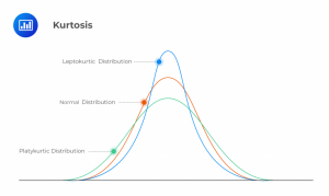
A data set would be described as Mesokurtic if it closely resembled a normal distribution, Leptokurtic if it was more tightly clustered around the mean, and Platykurtic if it is more widely distributed. The kurtosis of a normal distribution has a value of 3, so the excess Kurtosis is calculated as:
$$
Excess\quad Kurtosis=\left( \frac { \Sigma { \left( { X }_{ i }-X \right) }^{ 4 } }{ { s }^{ 4 } } \ast \frac { 1 }{ n } \right) -3
$$
$$ s=standard\quad deviation $$
$$ n=number\quad of\quad observations $$
Skewness is another way to describe the distribution of a data set. It refers to how symmetrical a data’s distribution is relative to a completely symmetrical normal distribution. A data set with negative skew has more values to the extreme left side of the distribution, and positive skew indicates the same occurring to the right side of the scale. Either of these conditions would be referred to as the distribution having “fat” tails.
$$ Skewness=\frac { \Sigma { \left( { X }_{ i }-X \right) }^{ 3 } }{ { s }^{ 3 } } \ast \frac { 1 }{ n } $$
There are several concepts involving calculating probabilities you need to know. Most of these involve determining the probability of multiple events occurring, given the probability of each individual event.
The Multiplication Rule applies to the joint probability of multiple events occurring. The formula is as follows:
$$ P\left( AB \right) =P\left( A|B \right) P\left( B \right) $$
The joint probability of both events happening (P(AB)), is the conditional probability of A, assuming B occurs (P(A|B)), times the probability of B (P(B)). Since the probability of both events happening is less than the odds of either one individually, the joint probability will always be lower than either input.
The Addition Rule applies to the probability of multiple events occurring, i.e., A and/or B occurs. That formula is:
$$ P\left( AorB \right) =P\left( A \right) +P\left( B \right) -P\left( AB \right) $$
Since both P(A) and P(B) include the possibility of both events occurring, we subtract the probability of both so that it’s not double-counted.
The Total Probability rule is similar to the addition rule but deals with the combination of conditional probabilities to create the entire probability of an event occurring. The sum of all conditional probabilities for an event adds up to the non-conditional probability of that event, if the conditions are mutually exclusive.
Two important concepts related to statistics in portfolio management are Correlation and Covariance. Correlation refers to the ratio of covariance between two variables and the product of their standard deviations. Covariance is the degree to which two variables move in sync with one another.
The formula to calculate the covariance of two assets (a and b) in a portfolio appears as follows.
$$ { \sigma }_{ { R }_{ a },{ R }_{ b } }=\sum _{ }^{ }{ P\left( { R }_{ a } \right) \left[ { R }_{ a }-E\left( { R }_{ a } \right) \right] } \left[ { R }_{ b }-E\left( { R }_{ b } \right) \right] $$
It is important to understand the nature of covariance, but you should not have to calculate this formula by hand on the exam. You should expect, however, to be calculating correlations, which use the following formula:
$$ Correlation\left( { R }_{ a },{ R }_{ b } \right) =\frac { Covariance\left( { R }_{ a },{ R }_{ b } \right) }{ StdDev\left( { R }_{ a } \right) \ast StdDev\left( { R }_{ b } \right) } $$
Be careful in exam questions involving these equations, because sometimes you will be given the portfolio risk expressed as the Standard Deviation or as the Variance. Don’t forget that the Standard Deviation is the square root of the Variance.
The Correlation value ranges between -1 and 1.
Bayes’ Formula is a method of calculating an updated probability of an event occurring, given a set of prior probabilities.
$$ P\left( { E }_{ i }|A \right) =\frac { P\left( { E }_{ i } \right) P{ \left( A|{ E } \right) }_{ i } }{ \Sigma P\left( { E }_{ j } \right) P\left( { A|E }_{ j } \right) } $$
$$ P\left( { E }_{ j } \right)=prior\quad probabilities $$
$$ A=an\quad event\quad known\quad to\quad have\quad occurred $$
$$ P\left( { E }_{ i }|A \right)=posterior\quad probability $$
There are several types of distributions you will need to understand, and this includes understanding a few common kinds of randomly distributed variables.
A Discrete Uniform Random Variable is one where the probabilities of all outcomes are equal, like the roll of a die. A Bernoulli Random Variable is one that can have only two outcomes. Similarly, a Binomial Random Variable is the number of specific outcomes in a Bernoulli situation that are independent of each other, such as the results of flipping a coin.
One way to calculate potential outcomes using a Bernoulli approach is known as a Binomial Tree:
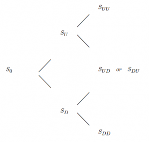
In this case, each final outcome is seen as successive iterations of Bernoulli events. At each point in time, the stock goes up or down. The tree lists all possible outcomes for this stock, and the probability of each final outcome is the multiplied product of the probability at each step along the way. A good way to catch potential errors when calculating the values of a binomial tree is that each column (a specific point in time) should add up to a probability of 100%.
The curriculum specifies several methods of tracking and managing risk exposures using quantitative means. An important one is known as Roy’s Safety-First Ratio. This is based on the principle that an optimal portfolio is one that minimizes the probability of a returning less than a given threshold level. Achieving a return less than a specified required return is known as Shortfall Risk. The Safety First Ratio is expressed as the excess return of the portfolio (expected returns – threshold returns) divided by portfolio risk (standard deviation):
$$ SF\quad Ratio=\frac { E\left( { R }_{ p } \right) -{ R }_{ L } }{ { \sigma }_{ p } } $$
Computing technology has introduced new methods of performance forecasting, including Monte Carlo Simulation. This method involves building a model of the portfolio and potential outcomes, then running a simulation of what could happen over time (factoring in all available probabilities and covariances of related variables) thousands of times. The output of this method is a distribution of the potential outcomes far more detailed than what a simple linear model could project. This is compared to the other common technique of Historical Simulation. In that approach, a projected portfolio is run through actual historical situations to see how it would have performed. This approach gives a much more limited set of outcomes than the Monte Carlo, but has the benefit of being based on observed market events rather than projected simulations.
A core tenet of statistics is using samples of data to find information about the entire population of a data set. It’s often impossible to gather all of the data of a population, so we rely on representative samples and try to make sure they properly represent the population from which they are drawn (like polls given to small groups of people to represent a whole state or country). One major assumption that underpins the validity of this approach is the Central Limit Theorem. This posits that a data sample will have a mean and variance that approach the mean and variance of the population it represents as the sample size becomes sufficiently large. It is widely accepted that a sample of size of at least 30 is usually enough to make the sample representative, but that can vary depending on the skewness of the sample distribution.
A common way (that will definitely appear multiple times on the exam) of analyzing the probability distribution of a data sample is to use the Student’s T-Distribution. This distribution is appropriate for small samples when the population variance is unknown. The formula for calculating a t-statistic is:
$$ t=\frac { x-\mu }{ \frac { S }{ \sqrt { n } } } $$
$$ x = sample \quad mean $$
$$ \mu =population\quad mean $$
$$ S=sample \quad standard \quad deviation $$
$$ n= sample \quad size $$
The t-distribution has an important parameter known as the Degrees of Freedom. The degrees of freedom is calculated as n-1. The t-distribution is symmetrical about its mean and has thicker tails than the normal distribution. The shape of the distribution is dependent on the number of degrees of freedom. As the number of degrees of freedom increases, the distribution becomes more closely gathered around the mean.
A big part of the statistics part of the curriculum deals with the use of Confidence Intervals. A confidence interval is the range of values in which a statistician believes that a certain population parameter lies. They incorporate a trade-off of value range and confidence, such that the smaller the area in which the value is believed to exist, the lower the confidence that it is actually there. There are three primary scenarios for calculating the confidence intervals in the CFA program curriculum.
1. A normal distribution with a known variance:
$$ CI=X\pm { z }_{ \frac { \alpha }{ 2 } }\ast \frac { \sigma }{ \sqrt { n } } $$
2. A normal distribution with unknown variance:
$$ CI=X\pm { t }_{ \frac { \alpha }{ 2 } }\ast \frac { S }{ \sqrt { n } } $$
3. A normal distribution with unknown variance and a sample size is large enough:
$$ CI=X\pm { z }_{ \frac { \alpha }{ 2 } }\ast \frac { S }{ \sqrt { n } } $$
When the population variance is known, we can use the more accurate z-score to determine the confidence interval instead of the student’s t-score, but the Central Limit Theorem allows us to also use the z-score when the sample size is large enough.
Hypothesis testing is a method of determining the statistical significance of a given data point in a distribution. There are One-Tailed Tests that test the possibility of a change in one direction, and Two-Tailed Tests regarding changes in both positive and negative directions. This method uses calculated test statistics to determine whether a given hypothesis should be accepted or rejected.
The test statistic for the hypothesis testis is calculated as follows:
$$ Test\quad statistic=\frac { Sample\quad statistic-Hypothesized\quad value }{ Standard\quad error\quad of\quad the\quad sample\quad statistic } $$
There are two types of errors that could occur when running a hypothesis test. Type 1 error occurs when we reject a true null hypothesis and Type 2 error occurs when we fail to reject a false null hypothesis. The level of significance (α) represents the probability of making a type 1 error.
Another important component of hypothesis testing is the P-Value. If the calculated P-value is lower than the level of significance, then we can reject the null hypothesis.
The correct hypothesis test for a normal distribution of the random variable is the Z-test, which is calculated as:
$$ z-statistic=\frac { X-{ \mu }_{ 0 } }{ \frac { \sigma }{ \sqrt { n } } } $$
$$ X=sample\quad mean $$
$$ { \sigma }_{ 0 }=Hypothesized\quad mean\quad of\quad the\quad population $$
$$ { \mu }=standard\quad deviation\quad of\quad the\quad population $$
$$ n= sample \quad size $$
For hypothesis testing a population mean when the population variance is unknown and the sample size is large, a T-test is more appropriate:
$$ { t }_{ n-1 }=\frac { X-{ \mu }_{ 0 } }{ \frac { s }{ \sqrt { n } } } $$
$$ X=sample\quad mean $$
$$ { \sigma }_{ 0 }=Hypothesized\quad mean\quad of\quad the\quad population $$
$$ { s }=standard\quad deviation\quad of\quad the\quad sample $$
$$ n= sample \quad size $$
Your testing materials will include tables of significant values for t- and z-scores, so that you can compare to them in determining whether a calculated value exceeds the level necessary to reject a null hypothesis.
For hypothesis testing to show whether the population correlation coefficient equals zero (absence of linear relationship between two variables), we use the t-statistic:
$$ t=\frac{r\sqrt{n-2}}{\sqrt{1-r^2}} $$
$$r = sample\quad correlation $$
$$ n = sample\quad size $$
The decision rule is to reject the null hypothesis (⍴=0)/to uphold the alternative hypothesis (⍴≠0) if t is greater than the critical value from the t-distribution table. Otherwise, we fail to reject the null hypothesis.
There are two classifications of statistical tests that you will need to know, Parametric and Non-Parametric. Parametric tests involve any testing where the given parameter follows a specific distribution. Non-parametric testing does not involve making any assumptions about the distribution of the parameter being studied. An instance where this could be necessary is when there are significant outliers that could cause the mean value of a dataset to be unrepresentative of the data. For this reason, if you wanted to run a test focused on the median of a dataset instead of the mean you would run a non-parametric test.
FRM Part 1 and Part 2 Complete Online Course
Access CFA Level I quantitative methods practice questions, mock exams, formula sheets, calculator tutorials, and structured revision tools designed to help you strengthen core concepts and improve exam-day accuracy with AnalystPrep’s study platform.
Offered by AnalystPrep


The CFA institute postponed the June exams and cancelled the December 2020 exams... Read More
If you are searching for the November 2025 CFA Level I exam results,... Read More

Get Ahead on Your Study Prep This Cyber Monday! Save 35% on all CFA® and FRM® Unlimited Packages. Use code CYBERMONDAY at checkout. Offer ends Dec 1st.
