


Currency Management for Emerging Marke ...
Managing emerging market currency risk presents a unique set of challenges, with two... Read More

When the yield curve is expected to remain unchanged, investors can capitalize on this scenario by incorporating either of the following strategies into their portfolios:
Moreover, you can explore a repo-carry trade, similar to the essential carry trade covered in other curriculum sections. This involves using repurchase agreements. The effectiveness of these approaches relies on the yield curve’s steady outlook matching the actual conditions when the investment horizon concludes.
Derivatives present an alternative strategy. They’re often more cost-effective than trading equivalent securities and offer straightforward management.
Among the concepts crucial for level III exam candidates is understanding futures. Calculating the correct number of futures contracts to incorporate into a portfolio for the desired exposure is significant. The formula for this calculation is:
$$ \text{Futures BPV} =\frac {\text{BPV}_{(CTD)} }{ \text{CF}_{(CTD)} } $$
Where:
\(BPV\) = Basis-point value.
\(CTD\) = Cheapest to deliver.
\(CF\) = Conversion Factor.
$$ \text{Swap BPV} = \text{Modified Duration of Swap} \times \frac {\text{Swap Notional Value} }{ 10,000} $$
A dynamic yield curve scenario encompasses a parallel shift in yields, wherein the interest rates across different maturities change equally. These situations present potential opportunities to generate alpha, which depends on the tools employed. The following graphics illustrate the yield curve’s downward and upward parallel shift.
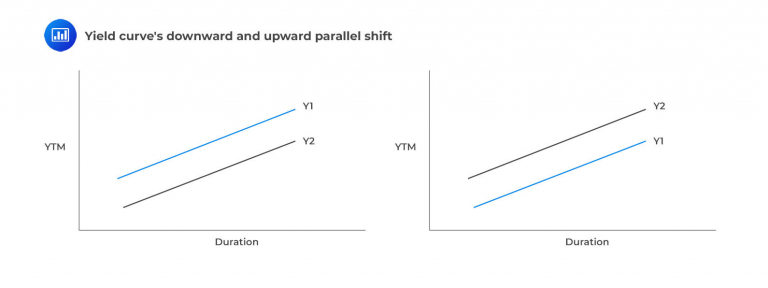
The following strategies are common ways to capitalize on a downward parallel shift in the yield curve:
In contrast to the previous section, which focused on parallel shifts in yield curves, this sub-section addresses different yield curve slope views. These views involve either a ‘flattening’ or ‘steepening’ yield curve. The ‘flattening’ scenario is illustrated in the graphic below.
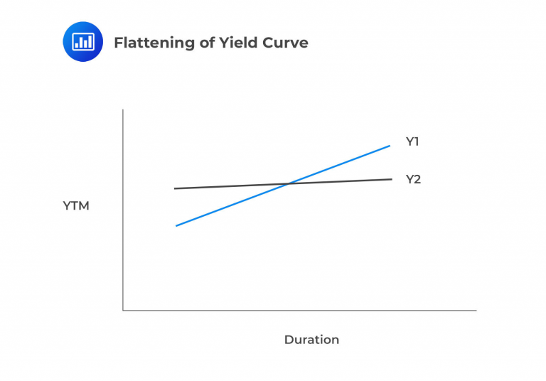
While an upward-sloping yield curve is standard in most economic conditions, a flattening yield curve signifies a decrease in long-term rates and an increase in short-term rates. This scenario often foreshadows financial distress. Typically, lenders expect higher compensation for the added risk associated with longer-term loans. This principle encounters challenges during a yield curve flattening.
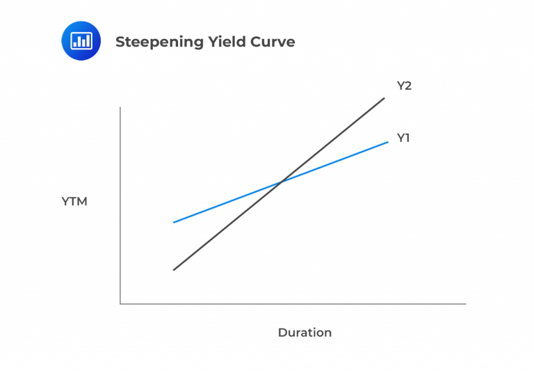
A yield curve steepening is the exact opposite, depicted below:
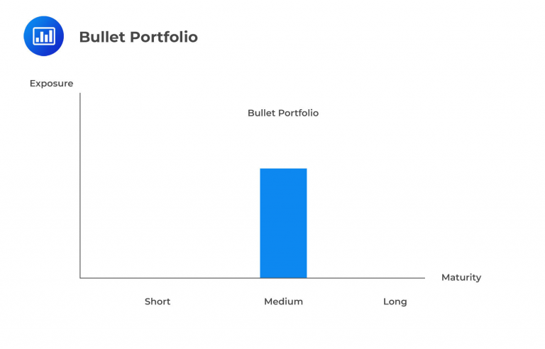
Managers expecting these ‘non-parallel shifts in the yield curve will often use barbell portfolios. A barbell has concentrations of duration in the long and short-term areas, as shown below:
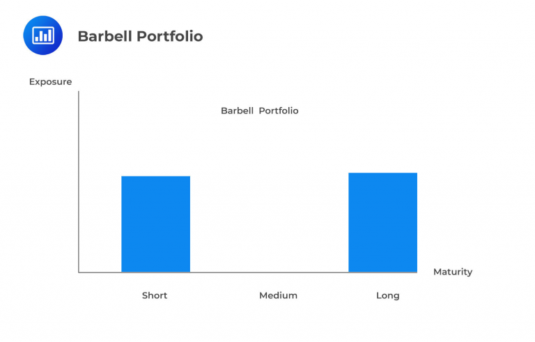
This barbell portfolio is expected to excel compared to other strategies when a yield curve flattens. Conversely, this approach could be shorted or merged with a long bullet portfolio during steepening to create a butterfly portfolio. The crucial factor in determining the optimal structure is comprehending that longer-term durations significantly influence portfolio performance. Consequently, when long-term yields decrease, the barbell portfolio gains substantial exposure to this duration level and is positioned to outperform a bullet portfolio.
Bull-steepening occurs when short-term yields experience a more significant decline compared to longer-term yields. This situation can result from actions taken by the central bank, such as reducing short-term rates to stimulate a sluggish economy. The appropriate strategy is to develop portfolios with a net positive duration.
A bear-steepening scenario occurs when long-term interest rates increase more than short-term rates. This often happens when higher economic growth and inflation expectations lead to higher long-term rates while short-term rates remain relatively stable.
In response to bear-steepening, a corresponding portfolio strategy involves reducing duration through short positions.
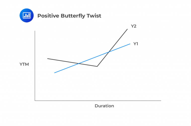
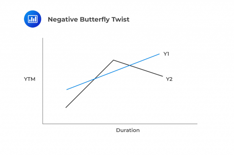
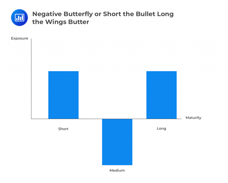
In contrast to the previous segments covering parallel and steepening/flattening yield curves, this section focuses on yield curve ‘twists.’ Twists represent fundamental duration movements but in a more straightforward manner. Instead of segmenting the duration spectrum into numerous points along the x-axis, butterfly twists divide it into three sections: short, intermediate, and long-term maturities (also labeled duration). As illustrated below, a positive butterfly twist reflects rising short-term and long-term rates while intermediate rates decrease. The negative butterfly twist is the reverse.
Butterfly strategies are a combination of a short bullet and long barbell or a long bullet and short barbell strategies, as depicted below:
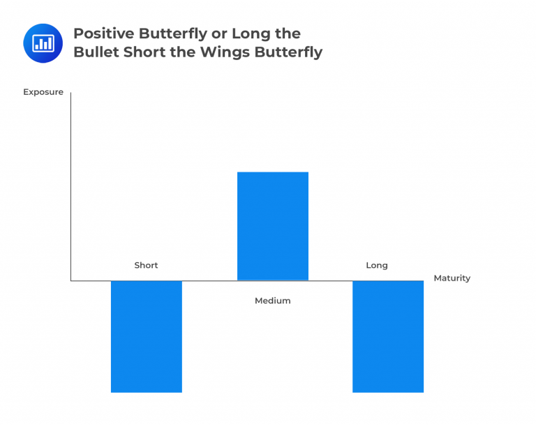
Candidates should be capable of evaluating yield curve expectations in the exam and suggesting a suitable butterfly strategy. Two crucial principles will aid candidates in making an intuitive recommendation:
Applying this rationale, investors should seek short exposure to that duration segment if they anticipate rising interest rates. Conversely, investors should consider going long in that section of the duration segment for an anticipated rate decrease.
This section focuses on bonds with embedded options, which managers often use to handle volatility. For instance, many US bonds, including mortgage-backed securities, have embedded options.
Derivatives can offer an efficient and swift way to adjust portfolio duration. Managers dealing in illiquid bonds with high trading costs might otherwise need to make multiple transactions to weak portfolio duration manually. Instead of buying and selling bonds, a single derivative transaction can often achieve the desired effect.
Furthermore, derivatives are valuable for non-parallel shifts since they allow the selection of specific interest points. This flexibility is particularly advantageous for making short-term tactical adjustments.
When the derivative portfolio has the exact cost and expected payoff as the adjusted underlying portfolio, the law of one price dictates that they are economically identical.
Options contracts exhibit inherent convexity, which applies to both the put and call sides. This characteristic stems from the fact that incorporating long call options enhances the potential upside of a portfolio while integrating long put options mitigates losses in adverse scenarios. As a result, portfolio managers can take the following actions:
Furthermore,
The following formulas prove valuable for portfolio managers quantifying and managing volatility-driven trading.
Effective Duration Formula:
$$ \frac {(PV_-) – (PV_+) }{ [2 \times (\text{Change in Curve}) \times (PV_0)] } $$
Effective Convexity Formula:
$$ \frac { (PV_-) + (PV_+) – 2(PV_0) }{ [(\text{Change in Curve}) \times (PV_0)] } $$
Where:
\(PV_-\) = Present value of the bond if interest rates decline.
\(PV_+\) = Present value of the bond if interest rates increase.
\(PV_0\) = Present value of the bond (initial).
Note: Each of these variables defined above relates to the same bond but is based on different times and outcomes.
Swaptions provide an additional avenue for managing volatility in bond portfolios. A swaption grants the holder the option to engage in an interest rate swap at a predetermined interest rate and within a specific investment period. Acquiring the right to enter either a payer or receiver swaption involves paying a premium to the swap counterparty, who acted as the trade facilitator or market maker. In the swap, one leg features a payment set at a fixed rate, while the other is tied to a floating or reference rate. Candidates are assumed to know the fundamental mechanics of interest rate swaps.
Pay fixed, receive floating\(\rightarrow\) Decreases portfolio duration.
Receiving fixed, paying floating \(\rightarrow\) Increases portfolio duration.
The notional principal of the swap is equal to:
Desired change in PVBP / PVBP of the swap
PVBP of the swap is the difference between the fixed and floating sides of the swaps’ PVBP.
Futures are frequently employed to modify portfolio duration based on the considerations outlined earlier. Managers aiming to alter portfolio duration should:
The number of contracts to be used is:
\(N_F\) = Desired change in PVBP / PVBP of a futures contract
And
\(\text{PVBP of futures contract} = \text{value} \times \text{modified duration} \times 0.0001\)
Key rate duration represents a portfolio’s responsiveness to specific interest rate changes. While curriculum examples often involve a limited number of key rates, like three years in total, in practical scenarios, these adjustments can occur more frequently based on the underlying bond maturities.
$$ {\text{Key Rate Duration}_\text{(for rate k)}} = \frac {-1}{PV} \times \left[ \frac {\text{Change(PV) }}{\text {Change rate}_{(k)}} \right] $$
Where:
\(PV\) = Present value of bond.
\(k\) = Rate at specific maturity being measured.
If accurately computed, key rate duration should yield the same outcome as effective duration. The advantage of conducting key rate analysis lies in its ability to provide insights into the overall duration of the measured portfolio and the specific periods where the risks are situated. In contrast, effective duration offers a general assessment of the portfolio’s response to a given rate change without this detailed information level, often called shaping risk.
When referring to crucial rate durations, we are discussing the sensitivity of a bond to interest rate changes when only one point on the yield curve shifts. These durations can be quantified regarding the Price Value of a Basis Point (PVBP).
Critical rate durations are commonly computed for multiple points along the yield curve. For instance, a particular bond might have critical rate durations assessed at the 2, 5, 7, 10, 20, and 30-year marks. If the bond’s critical rate duration at the 7-year point is 5.5, this indicates that a 1.00% increase in interest rates at the 7-year milestone would lead to a 5.5% decrease in the bond’s value.
Portfolio managers can use critical rate durations to predict how changes in interest rates will impact bond values. This involves adding up the expected interest rate movements multiplied by their durations at critical points along the yield curve.
Question
Which of the following statements best describes a bull-steepening of a yield curve?
- Any yield curve change that results in a positive fixed-income portfolio valuation change.
- A bull-steepening involves long-term yields-to-maturity rising more than short-term yields-to-maturity. This often happens due to increased long-term rates amid higher growth and inflation expectations while short-term rates remain stable.
- A bull-steepening is when long-term yields rise more than short-term yields.
Solution
The correct answer is C:
Bull-steepening occurs when long-term yields increase at a greater rate than short-term yields.
B is incorrect: It describes a bear-steepening.
A is incorrect: It describes a bullish scenario for a fixed-income investor but does not explicitly define a bull-steepening.
Reading 21: Yield Curve Strategies
Los 21 (b) Formulate a portfolio positioning strategy given forward interest rates and an interest rate view that coincides with the market view
Los 21 (c) Formulate a portfolio positioning strategy given forward interest rates and an interest rate view that diverges from the market view in terms of rate level, slope, and shape
Los 21 (d) Formulate a portfolio positioning strategy based upon expected changes in interest rate volatility
Los 21 (e) Evaluate a portfolio’s sensitivity using key rate durations of the portfolio and its benchmark
Offered by AnalystPrep


