Risk Management for Changing Interest Rates: Asset-Liability Management and Duration Techniques

After completing this reading, you should be able to:

• Discuss how asset-liability management strategies can help a bank hedge against interest rate risk.
• Describe interest-sensitive gap management and apply this strategy to maximize a bank’s net interest margin.
• Describe duration gap management and apply this strategy to protect a bank’s net worth.
• Discuss the limitations of interest-sensitive gap management and duration gap management.

How Asset-Liability Management Strategies Help a Bank to Hedge Against Interest Rate Risk

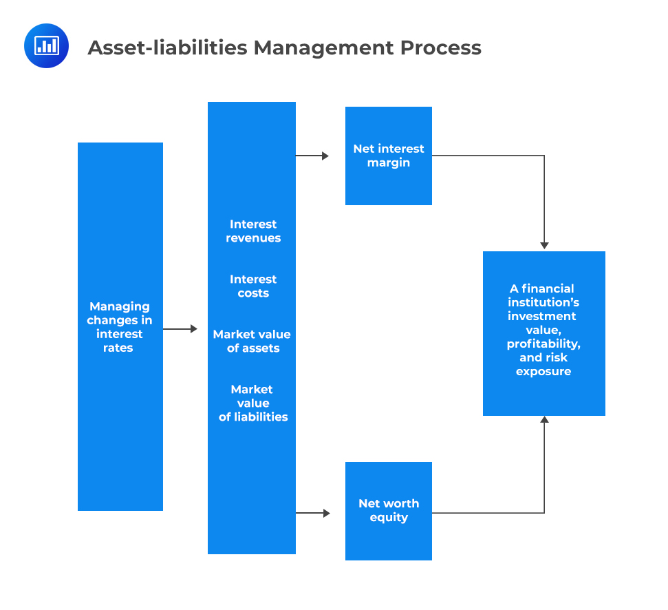
Asset-liability management (ALM) is utilized to control a bank’s sensitivity to changes in market interest rates and to limit losses in its net income or equity. Financial service managers should pay attention to an institution’s portfolio as a whole and how it contributes to the firm’s ultimate goal of sufficient profitability and allowable risk.

Asset-Liability Management Strategies

There are three asset-liability management strategies. These include:

1. Asset management strategy;
2. Liability management strategy; and
3. Funds management strategy.

i. Asset Management Strategy

Asset management strategy involves control over assets, but not control over liabilities. In other words, the bank’s management regulates the allocation of the bank’s assets but believes that the bank’s sources of funds, i.e., deposits, are outside its control.

ii. Liability management

Liability management entails the control over the bank’s liabilities, i.e., borrowed funds, by changing interest rates offered on the liabilities. Banks use this strategy to maintain a balance between the assets and liabilities’ maturities to maintain liquidity while at the same time facilitating lending, hence maintaining a healthy balance sheet.

iii. Funds management

Funds management strategy combines both asset and liability management strategies to achieve a balanced liquidity management strategy. The fund manager ensures that the maturity schedule for the deposits matches the demand for loans. The need to establish new sources of funds in the 1970s and risk management problems faced with troubled loans and volatile interest rates in the 1970s and 1980s led to the concept of planning and regulation over both sides of a bank’s balance sheet, thus the essence of funds management.

The following diagram illustrates asset-liability management in banking and financial services:

Interest Rate Risk

Interest rate risk is one of the primary and potentially most damaging forms of threats that all financial firms face. Fluctuations of interest rates have an impact on the balance sheet and the income statement as well as expenses on financial institutions.

Forces Determining Interest Rates

Loanable Funds Theory

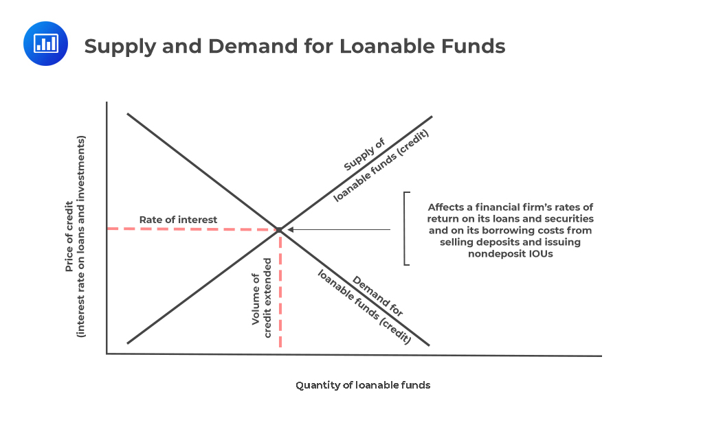
The level of market interest rates is a factor of supply and demand for credit. In other words, when the need for credit rises, the interest rates increase. On the other hand, a decline in the demand for money causes interest rates to decline. The converse is also true.

The following figure illustrates the determination of interest rates in the financial marketplace where the demand and supply of credit interact to set the credit price:

Inflation

Inflation also has an impact on the levels of interest rates. When the inflation rate is high, interest rates rise. This is because lenders demand higher interest rates to compensate for the decline in the purchasing power of the cash they will pay in the future.

Governments

The government plays a central role in determining how interest rates are impacted. Mainly, the Fed in the U.S. usually makes periodic announcements on how changes in monetary regulations are likely to influence interest rates. Thus, for survival, financial managers must be price takers and not price makers, as they have to accept interest rate levels as providers and plan as per the presented interest rate levels.

Financial firms typically face two main kinds of interest rate risk as the market interest rates move. These include:

1. Price risk: The market value of bonds or assets falls when interest rates rise.
2. Reinvestment risk: Falling interest rates make interest payments (coupons) of bonds to be reinvested at lower rates.

The Measurement of Interest Rates

Interest Rates are the Price of Credit

The interest rate refers to the proportion of the fees one is required to pay to acquire credit. Typically, this ratio is expressed in percentage format: \( \text {points and base points}\left( \cfrac { 1 }{ 100 } \text {of a percentage point} \right) \)

Yield to Maturity (YTM)

The yield to maturity is one of the most basic methods used in measuring rate. It is the approximate discount rate that equates the current market price of a loan with the expected stream of future income payments generated by the loan. It is also referred to as redemption yield or book yield.

Calculation of the Yield to Maturity

$$ \begin{align*} & \text{Current market price of a loan or security} \\ &=\cfrac {\text {Expected cash flow in Period 1} }{ { \left( 1+\text{YTM} \right) }^{ 1 } } \\ &+\cfrac {\text {Expected cash flow in Period 2} }{ { \left( 1+ \text{YTM} \right) }^{ 2 } } +\cdots \\ &+\cfrac {\text {Expected cash flow in Period n} }{ { \left( 1+ \text {YTM} \right) }^{ \text n } } \\ &+\cfrac {\text {Sale or redemption pricf security or loan in period n} }{ { \left( 1+ \text {YTM} \right) }^{ \text n } } \end{align*} $$

Example: Calculation of Yield to Maturity

Assume that a bond is purchased at $1,200. One is required to make level interest payments of $200 per annum over the next five years. If it is redeemed for $1,000 at maturity, what is the yield to maturity?

Solution

We need to find YTM such that the current price is equal to $1,200.

$$ \begin{align*} $1200 & =\cfrac { $200 }{ { \left( 1+ \text{YTM} \right) }^{ 1 } } +\cfrac { $200 }{ { \left( 1+ \text{YTM} \right) }^{ 2 } } +\cfrac { $200 }{ { \left( 1+ \text{YTM} \right) }^{ 3 } } +\cfrac { $200 }{ { \left( 1+ \text{YTM} \right) }^{ 4 } } \\ & +\cfrac { $200 }{ { \left( 1+ \text{YTM} \right) }^{ 5 } } +\cfrac { $1,000 }{ { \left( 1+ \text{YTM} \right) }^{ 5 } } \\ \end{align*} $$

To solve the above equation, we use a financial calculator with the variables: \(N=5\), \(PV=-1200\), \(PMT=200\) and \(FV=1000\) then hit \(CPT\) followed by \(I/Y\). You should be able to get 14.1529. Hence the YTM is 14.15%.

Bank Discount Rate

The bank discount rate refers to the interest rate quoted for short-term loans and money-market instruments such as treasury bills.

$$ \begin{align*} \text {Bank Discount Rate} \\ &=\left( \cfrac { 100- \text {Purchase price on loan or security} }{ 100 } \right) \\ &\times \left( \cfrac { 360 }{\text {Number of days to maturity} } \right) \end{align*} $$

The bank discount rate ignores the effect of compounding of interest and is based on a 360-day year, unlike YTM, which assumes a 365-day year and assumes that the interest income is compounded at the calculated YTM. Additionally, it utilizes the face value of a financial instrument to compute its yield/rate of return, which makes this method more straightforward but theoretically incorrect.

Under the bank discount rate, the purchase price of a financial instrument is used, instead of its face value, since it forms a better base in the calculation of the instrument’s exact rate of return.

Example: Bank Discount Rate

Assume that a treasury bill has a face value of $1,000 set for payment at maturity. Its purchase price is $97. If the security is to mature in 60 days, calculate the interest rate measured using the bank discount rate.

Solution

$$ \text{Bank Discount Rate}=\cfrac { \left( 100-97 \right) }{ 100 } \times \cfrac { 360 }{ 60 } =0.18=18\% $$

Converting a Bank Discount Rate to the equivalent YTM

$$ \text{YTM equivalent yield}=\cfrac { \left( 100-\text{Purchase Price} \right) }{\text {Purchase Price} } \times \cfrac { 365 }{\text {Days of maturity} } $$

Example: Converting a Discount Rate to YTM

Assume that a treasury bill has a face value of $1,000 set for payment at maturity. Its purchase price is $97. If the security is to mature in 60 days, calculate the yield to maturity equivalent yield.

Solution

$$ \text{YTM equivalent yield}=\cfrac { \left( 100-97 \right) }{ 97 } \times \cfrac { 365 }{ 60 } =0.1881,\text{ or }18.81\% $$

The Components of Interest Rates

Market interest rates are a function of:

1. The risk-free real rate of interest; and
2. Various risk premiums including default risk, inflation risk, liquidity risk, call risk, and maturity risk.

The market interest rate on a risky security or loan is given as the sum of risk-free real interest rate (inflation-adjusted return on government securities) and risk premiums to compensate lenders who accept risk to cover credit risk and liquidity risk, among other risks.

The risk-free real interest rate changes over time as a result of shifts in supply and demand for loanable funds, while risk premiums change over time as a result of “characteristics of the borrower,” the maturity of securities, and marketability.

Yield Curves

A yield curve is a graphical portrayal of the relationship between yields and maturities of securities. Generally, yield curves are established with treasury bonds to keep the credit (default) risk constant.

The yield curve comes in different shapes as follows:

1. An upward sloping curve shows that the long-term rates are higher relative to the short-term rates.
2. A downward sloping curve implies that the short-term rates are higher relative to the long-term rates.
3. The horizontal curve shows equal risk for long-term and short-term rates.

Essentially, financial institutions do much better with an upward-sloping yield curve. Mostly, lending organizations experience a positive maturity gap between the average maturity of their assets and liabilities in the following circumstances:

• If the yield curve is sloping upwards, thus, revenues generated from longer-term assets will be more than the expenses incurred from shorter-term liabilities.
• Typically, the outcome is a positive net interest margin. In other words, the interest revenues are more than the interest expenses.
• However, horizontal (relatively flat) or negatively sloping yield curve results in a minimal or even negative net interest margin.

Interest-Sensitive Gap Management and its Application in Maximization of a Bank’s Net Interest Margin

Aims of Interest Rate Hedging

One of the purposes of interest rate hedging is to protect the net interest margin. A bank’s management should hold a fixed net interest margin (NIM) to cushion the bank’s profits against severe interest rate fluctuations.

$$ \text {Net interest margin (NIM)}=\cfrac {\text {Net interest income} }{\text {Total earning assets} } $$

The net interest margin is the difference between the interest income/revenue from loans and investments and the interest expense on deposits and other borrowed funds.

Example: Net Interest Margin

Nineva is an international bank in the United States. It reports $10 billion in interest revenue from its loans and security investments and $6.7 billion for its interest expense incurred to attract borrowed funds. If the bank’s total earning assets are worth $65 billion, calculate the bank’s net interest margin.

Solution

$$ \text{NIM}=\cfrac { $10 \text{ billion}-$6.7 \text{ billion} }{ $65 \text{ billion} } \times 100=5.08\% $$

Interest-Sensitive (IS) Gap Management

The IS gap management strategy calls for the manager to perform an analysis of maturities and repricing opportunities linked to the bank’s interest-bearing asset, money market borrowings, and deposits. The IS gap management involves control over the difference between the volume of a bank’s interest-sensitive liabilities and interest-sensitive assets.

Notably, the gap management aims to ensure that for each period, the dollar amount of interest-sensitive (re-priceable) assets is equivalent to the dollar amount of interest-sensitive (re-priceable) liabilities. This way, a financial institution can hedge itself against interest rate fluctuations, regardless of the direction of the interest rate movement.

Re-priceable Assets and Liabilities

Re-priceable assets include short term loans that are almost maturing or are nearing repricing/renewal. Examples are household loans or variable rate business. For instance, if there is a rise in interest rates, the bank/lender is most probably going to reinvest or renew the newly released funds at a higher interest rate. They also include short-term securities that are issued by the government, which are about to mature.

On the other hand, re-priceable liabilities are money market deposits that are almost maturing in which customers and firms have to negotiate for new deposit interest rates. An example is the floating rate deposits.

Interest Sensitive Gap

A gap exists between the interest-sensitive assets and liabilities in a situation where the re-priceable assets and re-priceable liabilities are not equal.

$$ \text {Interest sensitive gap} =\text {Interest sensitive assets}-\text {Interest sensitive liabilities} $$

Negative Interest Sensitive Gap

A ratio that is less than one, or a negative gap, comes about when the volume of a bank’s interest-sensitive liabilities is more than that of the interest-sensitive assets.

$$ \text {Interest sensitive gap} =\text {Interest sensitive assets}-\text {Interest sensitive liabilities} < 0 $$

Since in a negative gap the interest-sensitive assets are less than the interest-sensitive liabilities, there exists a risk in that if the interest rates rise, there will be losses as the bank’s net interest margin will reduce.

A defensive strategy can be applied to eliminate an adverse bank’s interest-sensitive gap. Management at the bank can do one of the following:

• Shortening the maturities of assets or lengthening the maturities of liabilities; or
• Decreasing interest-sensitive liabilities or increasing interest-sensitive assets.

Positive Interest Sensitive Gap

A ratio higher than one or a positive gap comes about when a financial institution’s interest rate sensitive assets are more than its sensitive interest liabilities.

$$ \text {Interest sensitive gap} =\text {Interest sensitive assets}-\text {Interest sensitive liabilities} > 0 $$

Since a positive gap implies interest-sensitive assets outweigh interest-sensitive liabilities, the associated risk is losses in case of a decline in interest rates as the bank’s net interest margin will fall.

A bank can employ a defensive strategy to eliminate a positive gap by:

• Extending the maturities of assets or shortening the timelines of liabilities; or
• Reducing interest-sensitive assets or increasing interest sensitive liabilities.

Measuring the Interest-Sensitive Gap (IS GAP)

Dollar IS GAP

The dollar IS GAP is the difference between the interest-sensitive assets (ISA) and interest-sensitive liabilities (ISL).

$$ \text {Dollar IS GAP=ISA-ISL} $$

An institution is said to be asset-sensitive if it has a positive dollar IS GAP while it is liability-sensitive if it has a negative dollar IS GAP.

Example: Dollar IS GAP

Prime bank’s interest-sensitive assets have a value of $300, and its interest-sensitive liabilities are worth $250. Calculate the dollar IS GAP.

Solution

\( \text {Dollar IS GAP} = $300-$250=$50 \)

Relative IS GAP Ratio

$$ \text {Relative IS GAP ratio}=\cfrac {\text {IS GAP} }{\text {Total Assets} } $$

A financial firm is asset-sensitive when the relative IS GAP is greater than Zero while it is liability sensitive when its relative IS GAP is less than zero.

Interest Sensitivity Ratio

$$ \text {Interest Sensitive Ratio}(\text {ISR})=\cfrac {\text {ISA} }{\text {ISL} } $$

Where \(ISA\) is the interest-sensitive assets; and

\(ISL\) is interest-sensitive liabilities.

Example: Interest Sensitivity Ratio

Prime bank’s interest-sensitive assets have a value of $300 million, and its interest-sensitive liabilities are worth $250 million. Calculate the interest-sensitive ratio of the bank.

Solution

$$ \text {Interest Sensitive Ratio}(\text {ISR}) =\cfrac {\text {ISA} }{\text {ISL} }=\cfrac { $300 }{ $250 } =1.2 $$

If ISR is < 1, then this is a liability-sensitive firm, while a firm whose ISR is > 1 is referred to as an asset-sensitive firm. A financial firm is said to be relatively insulated from interest rate risk if its interest-sensitive assets are equal to the interest-sensitive liabilities.

Computer-Based Techniques

The majority of the firms are using computer-based techniques where they have their liabilities and assets categorized as per their repriceable dates either weekly or in the next 30 days (monthly) and so on. An institution’s management attempts to have the bank’s sensitive interest assets matched with its interest-sensitive liabilities in each maturity bucket to have better chances of improving the institution’s financial earning objectives.

For instance, assume the latest computer run of a firm might indicate as follows.

$$ \begin{array}{l|c|c|c|c} \textbf{Maturity Buckets} & \bf {\text{Interest} \\ \text{Sensitive} \\ \text{Assets}} & \bf {\text{Interest} \\ \text{Sensitive} \\ \text{Liabilities}} & \bf {\text{Size of} \\ \text{Gap}} & \bf {\text{Cumulative} \\ \text{Gap}} \\ \hline {\text {1 day (next 24 hours)}} & {$56} & {$34} & {+22} & {+22} \\ \hline {\text {Day 2- 7}} & {140} & {180} & {-40} & {-18} \\ \hline {\text {Day 8-30}} & {78} & {67} & {+11} & {-7}\\ \hline {\text {Day 31-90}} & {300} & {240} & {+60} &{+53}\\ \hline {\text {Day 91-120}} & {435} & {356} & {+79} & {+132} \\ \end{array} $$

The computer runs to assist the firm to have a clear understanding of its actual interest-sensitive position.

For instance, in the above example, it has a positive gap in the next 24 hours. Thus, the firm’s earnings will improve if there is a rise in the interest rate between today and tomorrow. However, on the 2nd to the 30th day, the cumulative gap registered is negative, meaning if there is a rise in the market interests’ rates, interest expenses will increase by more than interest revenues. The remainder of the maturity bucket seems to fare well in case any interest rate rises since the cumulative gap turns out as a positive.

Interest-Sensitive (IS) in maximizing a Bank’s Net Interest Margin (NIM)

We calculate an institution’s net interest income to gauge how it will change following a rise in interest rates. The net interest income is derived as follows:

$$ \begin{align*} \textbf {Net Interest Income} &= \text {Total Interest Income}- \text{Total Interest Cost} \\ &=[\text {Average Interest Yield on rate sensitive assets} \\ &\times \text {Volume of rare sensitive assets} \\ &+\text {Average Interest Yield on Fixed}\left( \text {non-rate Sensnitive assets} \right) \\ &\times \text {Volume of Fixed Assets}]- [ \text {Average interest cost on rate} \\ &-\text {sensitive liabilities}\times \text {Volume of interest sensitive liabilities} \\ &+\text{Average interest cost on fixed (non-rate} \\ &-\text {sensitive) liabilities} \\ &\times \text {Volume of fixed (non-rate-sensitive) liabilities}] \end{align*} $$

Example: Net Interest Income

Suppose that a hypothetical bank has an average yield on rate-sensitive and fixed assets of 9% and 10%, respectively. Additionally, the bank has rate-sensitive and non-rate-sensitive liabilities cost of 7% and 6%, respectively.

During the coming week, the bank holds $2,000 million in rate-sensitive assets and $2,100 million in rate-sensitive liabilities. Assume that the asset total is 5,000. Further, suppose that these annualized interest rates remain steady.

Calculate the firm’s net interest income on an annualized basis.

Solution

$$ \text {Net interest income on an annualized basis}=0.09\times $2,000+0.10\times [5,000-  2,000] \\ -0.07\times $2,100-0.06\times \left[ 5,000-2,100 \right] =$159 \text { million}$$

Assuming that the market interest rate on rate-sensitive assets rises to 11% and the interest rate on rate-sensitive liabilities rises to 9% during the first week, this liability-sensitive institution will have an annualized net interest income of:

$$ \text {Net interest income on an annualized basis}=0.11\times $2,000+0.10\times \left[ 5,000-2,000 \right] \\ -0.09\times $2,100-0.06\times [5,000 – 2,100] = $157 \text{ million} $$

Thus, this bank will lose $2 million in net interest income on an annualized basis if market interest rates rise in the coming week.

Weighted Interest-Sensitive Gap

Suppose that National Bank currently has the following interest-sensitive assets and liabilities on its balance sheet:

$$ \begin{array}{lc|c|cc|c} \bf{ \text{Interest-} \\ \text{Sensitive} \\ \text{Assets}} & {} & \bf {\text{Interest-Rate} \\ \text{Sensitivity} \\ \text{Weight} \\ \text{(Assets)}} & \bf{ \text{Interest-} \\ \text{Sensitive} \\ \text{Liabilities}} & {} & \bf {\text{Interest-Rate} \\ \text{Sensitivity} \\ \text{Weight} \\ \text{(Liabilities)}} \\ \hline {\text {Federal} \\ \text{Fund} \\ \text{Loans)}} & {$75} & {1.51} & { \text{Interest-} \\ \text{bearing} \\ \text{deposits}} & {$275} & {0.87} \\ \hline {\text {Security} \\ \text{holdings}} & {$52} & {1.23} & { \text{Money-} \\ \text{market} \\ \text{borrowings}} & {$87} & {0.94} \\ \hline {\text {Loans} \\ \text{and} \\ \text{Leases}} & {$320} & {1.56} & {} & {} & {} \end{array} $$

Use the information to calculate the weighted interest-sensitive gap.

Solution

$$ \begin{align*} &\textbf {Weighted Interest Sensitive Gap} \\ &=(\text {InterestSensitiveAssets} \\ &\times \text{Interest Rate Sensitivity Weight for Assets}) \\ &-(\text {Interest Sensitive Liabilities} \\ &\times \text {Interest Rate Sensitivity Weight for Liabilities}) \end{align*} $$

Thus,

$$ \begin{align*} \textbf {Weighted Interest Sensitive Gap} = & [( 75\times 1.51 ) +( 52\times 1.23 ) +(320\times 1.56)] \\ & [( 275\times 0.87) +( 87\times 0.94)] \\  = & $355.38  \end{align*} $$

The Cumulative Gap

The cumulative gap is an overall measure of interest rate exposure. It is the total difference between repriceable assets and liabilities over a specified period. We can calculate the approximate impact of market interest rate fluctuations on the net interest income.

$$ \begin{align*} & \text {Change in net interest income} \\ &=\text {Total change in interest rate}\left( \text {Percentage points} \right) \\ &\times \text {Size of cumulative gap in dollars} \end{align*} $$

Duration Gap Management and its Application to Protect a Bank’s Net Worth

Duration gap management is a managerial tool used in insulating a firm’s net worth from serious implications of interest rates. Using duration as an asset-liability management tool is better relative to using interest-sensitive gap analysis. This is because the interest-sensitive gap only looks at the effects of changes in the interest rates on the bank’s net income and fails to take into account the impact of interest rate changes on the market value of the bank’s equity capital position. However, duration provides a single number, which makes it possible for the banks to be aware of the overall exposure to interest rate risk.

Definition of Duration

Duration refers to the value and time-weighted measure of maturity that considers the timing of cash inflows from earning assets and cash outflows related to liabilities. It primarily measures the mean maturity of expected future cash payments. In other words, it calculates the average time required to recover finances directed towards a particular investment.

The formula for calculating the duration is as follows:

$$ \text {D}=\cfrac { \sum_{\text t=1 }^{\text n }{\text { Expected CF in period t}\times \cfrac {\text {Period t} }{ { \left( 1+ \text {YTM} \right) }^{\text {t} } } } }{\text {Current Market Value or Price} } $$

Where the current market value or price is given by:

$$ \cfrac {\text {Expected cash flow in period t} }{ { \left( 1+ \text {YTM} \right) }^{\text {t} } } $$

Example: Duration

Assume that a bank gives a loan to a customer to be repaid in 5 years. The customer promises the bank an annual interest payment of 8% per annum. The par value of the loan is $2,000, which is also its price because the loan’s current yield to maturity is 8%.

Calculate the loan’s duration.

Solution

$$ {\text {D} }_{\text {loan} }=\cfrac { \sum _{ \text t=1 }^{ 5 }{ $160 } \times \cfrac { 5 }{ { \left( 1.08 \right) }^{ 5 } } +\left( 2,000\times \cfrac { 5 }{ { \left( 1.08 \right) }^{ 5 } } \right) }{ $2,000 } $$

This can be computed easily as in the following table:

$$ \begin{array}{l|c|c|c|c|c|c} \textbf{Year} & \textbf{1} & \textbf{2} & \textbf{3} & \textbf{4}  & \textbf{5} & \textbf{Total} \\ \hline {\text {Payment}} & {148.15} & {274.35} & {381.04} & {470.42} & {544.47+6,805.83} & \textbf{8,624.26} \\ \end{array} $$

$$ {\text {D} }_{\text {loan} }=\cfrac { $8,624.26 }{ $2,000 } =4.31 \text { years} $$

Duration as a Risk-Management Tool

The net worth (NW) a business is equivalent to the value of its assets less the value of its liabilities.

$$ \text {Net Worth (Equity)} = \text {Asset} -\text {Liabilities} $$

The value of an institution’s assets and liabilities change as the market interest rates changes, resulting in a change in its net worth.

$$ \text {Change in Net Worth} = \text {Change in Assets}-\text {Change in Liabilities} $$

According to portfolio theory, an increase in the market interest rates results in the market value (price) of both fixed-rate liabilities and assets to decrease. Additionally, when a financial firm’s maturity of liabilities and assets is longer, they are more likely to decrease in market value (price) when there is a rise in market interest rates.

Management can balance the average maturity of the anticipated assets cash inflows with the average maturity of the expected cash outflows related to liabilities by use of the equation of assets and liability durations. Therefore, duration analysis is applied in stabilizing, or immunizing the market price (value) of a financial organization’s net worth.

Price Sensitivity

One of the crucial characteristics of duration in the perspective of risk management is that it measures a financial instrument’s market value sensitivity to changes in interest rate.

$$ \cfrac {\text {Change in Price} }{\text {Price} } =-\text{D}\times \cfrac {\text {Change in Interest rate} }{ \left( 1+\text{i} \right) } $$

Where \( \frac {\text {Change in Price} }{\text {Price} }\)represents the percentage change in the market price

\(\frac {\text {Change in Interest rate} }{ \left( 1+\text{i} \right)}\)refers to the relative change in interest rates related to the asset or liability.

D is the duration, and the negative sign attached to D implies that market prices and interest rates of financial instruments move in opposite directions.

Example: Price Sensitivity

Assume that a firm holds a bond with a duration of 5 years and a price of $2,000. The market interest rates associated with this bond currently stand at 8%. Recent forecasts show that the interest rates may rise to 9%.

Calculate the percentage change that is expected to occur in the market value of the bond.

Solution

$$ \begin{align*} &\cfrac {\text {Change in P} }{\text {P} } =-\text {D}\times \cfrac {\text {Change in Interes trate} }{ \left( 1+\text {i} \right) } \\ & \cfrac {\text {Change in P} }{\text {P} } =-5 \text { years}\times \cfrac { \left( 0.09-0.08 \right) }{ 1.08 } =-4.63\% \end{align*} $$

Convexity and Duration

Convexity is a key term related to duration, and it captures the relationship between an asset’s change in price and its change in the interest rate or yield. Thus, it highlights the presence of a nonlinear relationship between changes in an asset’s price and changes in market interest rates.

It incorporates a number designed to assist portfolio managers in controlling and measuring the market risks in portfolio assets. Usually, a portfolio or an asset consisting of low duration and low convexity indicates a relatively small market threat. An increase in asset duration implies an increase in convexity.

This means that the rate of change in any interest-bearing asset’s price for a particular interest rate varies depending on the prevailing interest rates level.

Using Duration to Hedge against Interest Rate Risk

Financial institutions interested in fully hedging themselves from interest rate changes should choose assets and liabilities such that the duration gap is made as close to zero as possible. That is:

$$ \textbf {Duration gap} =\text {Dollar-weighted duration of Assets } – \text {Dollar-weighted Duration of Liabilities } \approx 0  $$

Since the dollar volume of assets usually is more than the dollar volume of liabilities, a financial firm purposing to minimize the implications of interest rate fluctuations must adjust for leverage:

$$ \begin{align*} \textbf {Leverage Adjusted Duration Gap} = \text {Dollar-weighted duration of Assets}-\\ \text{Dollar-weighted Duration of Liabilities}\times \cfrac { \text {Total Liabilities} }{\text {Total Assets} } \end{align*} $$

This implies that liabilities values must change more relative to the cost of assets to do away with a financial institution’s entire interest-rate threat exposure. Thus, the more significant the leverage-adjusted duration gap, the more sensitive the net worth (equity) of the firm to the changes in interest rates.

$$ \begin{align*} &\textbf {Change in the value of a firm’ s net worth} \\ &=[-\text {Average duration of assets}\times \cfrac {\text {Change in interest rate} }{ \left( 1+\text {Original discount rate} \right) } \times \text {Total Assets}] \\ &-[-\text {Average duration of liabilities} \times \cfrac {\text { Change in interest rate } }{ \left( 1+ \text{ Original discount rate } \right) } \times \text{Total Liabilities}] \end{align*} $$

Example 1: Change in the Value of a Firm’s Net Worth

Suppose that a financial institution’s average duration of its assets is five years. Additionally, the mean liability duration of the firm is six years, and the total liability of the firm is $250m, while its total assets are worth $380m. The initial interest rate was 8% but suddenly increased to 11%.

Calculate the change in the value of the firm’s net worth.

Solution

$$ \begin{align*} &\text {Change in the value of net worth} \\ &=\left[ -5\times \cfrac { 0.03 }{ \left( 1+0.08 \right) } \times 380 \right] -\left[ -6\times \cfrac { 0.03 }{ \left( 1+0.08 \right) } \times 250 \right] =-$11.11 {\text m} \end{align*} $$

Example 2: Dollar-weighted Asset Portfolio Duration

Assume that a bank holds assets with duration and market values as given the following table:

$$ \begin{array}{l|c|c} \textbf{Assets Held} & \bf { \text{Estimated Market} \\ \text{Values of Assets}} & \textbf {Asset Duration (Years)} \\ \hline {\text {Consumer loans}} & {129} & {8.65} \\ \hline {\text {Treasury bonds}} & {89} & {1.34} \\ \hline {\text {Consumer loans}} & {65} & {4.75} \\ \hline {\text {Real estate loans}} & {34} & {2.87} \\ \end{array} $$

Calculate the dollar-weighted asset portfolio duration for this firm.

Solution

$$ \textbf{DW asset portfolio duration} = \cfrac { \left( 8.65\times $129 \right) +\left( 1.34\times $89 \right) +\left( 4.75\times $65 \right) +\left( 2.87\times $34 \right) }{ \left( $129+$89+$65+$34 \right) } =5.1780  \text{ years}$$

Example 3: Calculating the Duration of a Bank’s Assets and Liabilities

The following tables represent a part of ABC Bank’s balance sheet:

$$ \begin{array}{l|c|c|c} \textbf{Asset Composition} & \bf {\text{The market value} \\ \text{of Assets} ($ \text M)} & \bf {\text{Interest Rate} \\ \text{of Assets}} & \bf {\text{Average. Duration} \\ \text{Assets (Years)}} \\ \hline {\text {U.S. Treasury securities}} & {400} & {12.00\%} & {5.45} \\ \hline {\text {Commercial loans}} & {120} & {8.00\%} & {2.34} \\ \hline {\text {Municipal bonds}} & {230} & {12.00\%} & {1.23} \\ \hline {\text {Total}} & {\textbf {750}} & {} & {} \\ \end{array} $$

$$ \begin{array}{l|c|c|c} \bf{\text{Liability} \\ \text{Composition.}} & \bf {\text{The market value} \\ \text{of Liabilities} ($ \text M)} & \bf {\text{Interest Rate} \\ \text{of Liabilities}} & \bf {\text{Average. Duration} \\ \text{Liabilities (Years)}} \\ \hline {\text {Negotiable CDs}} & {200} & {4.56\%} & {3.45} \\ \hline {\text {Other time deposits}} & {120} & {12.00\%} & {2.56} \\ \hline {\text {Subordinated notes}} & {100} & {8.00\%} & {1.54} \\ \hline {\textbf {Total Liabilities}} & {\textbf {420}} & {} & {} \\ \hline {\text {Stockholders’ equity}} & {\text {330}} & {} & {} \\ \hline \bf{\text {Total Equity and} \\ \text{Liabilities}} & {\textbf {750}} & {} & {} \\ \end{array} $$

Using the above tables,

i. Calculate the average duration of assets and liabilities.

The average duration of assets:

$$ \cfrac { 400 }{ 750 } \times 5.45+\cfrac { 120 }{ 750 } \times 2.34+\cfrac { 230 }{ 750 } \times 1.23=3.658266667= 3.658 \text{ years} $$

The average duration for liabilities:

$$ \cfrac { 200 }{ 420 } \times 3.45+\cfrac { 120 }{ 420 } \times 2.56+\cfrac { 100 }{ 420 } \times 1.54=2.741 \text { years} $$

ii. Calculate the current leverage-adjusted duration gap.

$$ \begin{align*} &\text {Current Leverage-adjusted duration gap} \\ &=\text {Average Asset suration}-\text {Average liability duration} \times \cfrac {\text {Total Liabilities} }{\text {Total Assets} } \\ &=3.658-2.741\times \cfrac { 420 }{ 750 } = +2.123 \text { years} \end{align*} $$

iii. Calculate the change in the value of net worth if the interest rates for both liabilities and assets register a rise from 7% to 10%.

$$ \text {Change in value of net worth}=-{ \text D }_{ \text A }\times \cfrac { \Delta { \text r} }{ \left( 1+ \text r \right) } \times { \text A}-\left[ -{ \text D }_{ \text L }\times \cfrac { \Delta r }{ \left( 1+ \text r \right) } \times { \text L} \right] $$

$$ \begin{align*} &\text {Change in value of net worth} \\ &=-3.658\times \cfrac { \left( +0.03 \right) }{ \left( 1+0.07 \right) } \times 750-\left[ -2.741\times \cfrac { \left( +0.03 \right) }{ \left( 1+0.07 \right) } \times 420 \right] \\ &=-44.643 \text {m} \end{align*} $$

This institution’s net worth would fall by approximately $44,643 million if interest rates increased by 3 percentage points.

Limitations of Interest-Sensitive Gap Management and Duration Gap Management

Limitations of Interest-Sensitive GAP Management

• The interest paid on liabilities tends to move much faster as compared to the interest rates earned on assets, thus leaving financial institutions with interest-rate threat exposure.
• It is quite hard to identify the repricing point of some liabilities and assets.
• The interest-sensitive gap fails to put into consideration the implications of interest rate fluctuations on the positions of equity.
• There is a basis risk that refers to the interest rates associated with assets of different kinds changing by different volumes and varied speed as compared to the interest rates of liabilities.
• Interest paid on liabilities fluctuates much faster relative to the interest earned on assets.

Limitations of Duration Gap Management

• It is hard to find liabilities and assets of the same duration.
• Some liabilities and assets may fail to have well a defined pattern of cash flows, thus, making it difficult to calculate the duration.
• Customer prepayments of loans might distort the anticipated cash inflows in a particular duration.
• Also, the expected cash inflows in duration can be disrupted by the customers defaulting payments (credit risk).
• The duration gap approach assumes that there is the existence of a linear relationship between the market value of liabilities and assets and interest rates, which is not entirely true.

Practice Question

National Bank has a cumulative gap for the coming year of +$128 million. The interest rates are expected to decrease by one and a half percentage points.

What is the expected change in the Bank’s net interest income?

A. -1.23 million

B. -1.92 million

C. 1.89 million

D. 128 million

The correct answer is B.

$$\begin{align*} &\text { Change in net interest income } \\ &= \text { Total change in interest rate}\left( \text {Percentage points} \right) \\ &\times \text {Size of cumulative gap in dollars}. \end{align*}$$

Thus,

$$\text {Expected change in net interest income}=$128 \text { million}\times \left( -0.015 \right) =-1.92 \text { million}$$