


Due Diligence.
When General Partners (GPs) consider making a long-term, illiquid investment in private equity,... Read More

Fixed-income portfolio managers often aim to maximize returns by purchasing securities with a higher Yield to Maturity (YTM) and a lower equivalent price than a comparable default risk-free government bond. For instance, if a U.S. Treasury bond offers a 2% YTM, a manager might seek a corporate bond with a 3% YTM and a lower price. The excess return targeted by these managers is encapsulated in the fourth term of the fixed-income return equation.
\( E(R) \approx \text{Coupon income} \)
\(+/− \text{Rolldown return}\)
\(+/− E (\Delta \text{Price due to investor’s view of benchmark yields})\)
\(+/− E (\Delta \text{Price due to investor’s view of yield spreads})\)
\(+/− E (\Delta \text{Price due to investor’s view of currency value changes})\)
Here, \(E(R)\) represents the expected return, \(\Delta\) denotes change, and the terms in the brackets represent different factors influencing the return.
Yield spreads between a specific bond and a comparable government bond, though not directly observable, are inferred from market data. These spreads serve as a risk premium, compensating investors for taking on credit and liquidity risks.
Active fixed-income portfolio managers must account for trading costs when calculating expected excess returns and implementing credit strategies.
The yield spreads over default risk-free government bonds primarily serve as a compensation for investors against the potential risk of not receiving the promised cash flows due to issuer default and the severity of loss if such a default occurs. These spreads can vary significantly across different ratings categories and time periods.
Consider the yield spreads as a percentage of total Yield to Maturity (YTM) for A-, BBB-, and BB rated US corporate issuers from mid-2009 to mid-2020. On average, 60% of total YTM was attributable to yield spread for BB rated issuers as compared to 33% for A rated issuers over the period. This percentage was at its lowest for all rating categories in 2010 as the US economy was recovering from the 2008–09 financial crisis. It reached its peak in early 2020 during the economic slowdown caused by the COVID-19 pandemic. The higher average proportion of all-in yield attributable to credit risk necessitates a greater focus on this factor among high-yield investors over the credit cycle.
The Credit Valuation Adjustment (CVA) framework evaluates the present value of credit risk for various financial obligations such as loans, bonds, and derivatives and is widely used by financial institutions to assess the risk of loans issued to businesses, among other financial commitments.
Default risk refers to the likelihood that a borrower will not fulfill their financial commitments, potentially leading to financial difficulties that prevent them from making scheduled loan repayments. Loss severity measures the potential loss a lender faces if a borrower defaults, indicating the unrecoverable amount in a defaulted loan.
The one-period credit spread estimate, which quantifies credit risk by combining the Loss Given Default (LGD) and the Probability of Default (POD), provides insights into the risk associated with different bond types. Historical rates of POD and LGD show typically lower rates for investment-grade bonds and higher rates for high-yield bonds. Additionally, global annual corporate default rates, which tend to rise during economic downturns, offer a broader overview of credit risk in the corporate sector, highlighting the increased likelihood of defaults under economic stress.
When discussing credit risk, two key aspects come into play: default and credit migration. For instance, a company like Enron, which was once a high-rated bond issuer, defaulted, which is a rare occurrence. However, credit migration, which refers to changes in the relative assessment of creditworthiness, happens more frequently. An example of this is when Moody’s downgraded Ford’s credit rating in 2019, which negatively impacted its bond prices. This is because the likelihood of a downgrade often exceeds that of an upgrade, and the yield spread increase at lower credit ratings is typically greater than the spread decrease in the event of a credit upgrade.
Investors, like those investing in Apple Inc., categorize credit risk using public debt ratings, distinguishing between investment-grade and high-yield market segments. Investment-grade bonds, like those of Apple Inc., generally have higher credit ratings, lower default risk, and higher recovery in the event of default, and offer lower all-in yields to maturity. Conversely, high-yield bonds, like those of a startup company, usually have higher yields to maturity due to lower (sub-investment or speculative grade) credit ratings, higher default risk, and lower recovery in the event of default.
In yield curve strategies, changes in the level, slope, and shape of the government bond term structure across maturities are established as primary risk factors. For instance, during the 2008 financial crisis and the COVID-19 pandemic in 2020, lower-rated bonds, like those of Lehman Brothers, faced a greater impact from these adverse market events, as evidenced by the widening gap between BBB rated and high-yield bonds.
Active portfolio managers often employ strategies based on credit spread curves, similar to benchmark yield curve strategies. These curves, categorized by rating, issuer type, or corporate sector, are derived from the difference between all-in yields to maturity for bonds within each category and a government benchmark bond or swap yield curve. Adjustments are made for specific credit spread measures.
For example, consider the decline in option-adjusted spreads for US BBB rated health care companies from Q3 2019 to Q3 2020. A bar graph would illustrate the decrease for each maturity. The primary credit risk factors for a specific issuer include the level and slope of the issuer’s credit spread curve. Ignoring liquidity differences across maturities, an upward-sloping credit spread curve suggests a relatively low near-term default probability that rises over time. Conversely, a flatter credit spread curve indicates equal likelihood of downgrade/default in the near- and long-term.
The credit spread curve is largely influenced by the credit cycle, which is the expansion and contraction of credit over the business cycle. This results in asset price changes based on default and recovery expectations across maturities and rating categories. Lower-rated issuers tend to experience greater slope and level changes over the credit cycle, including more frequent inversion of the credit curve, due to their larger rise in annual credit losses during economic downturns.
When it comes to bond pricing, credit spreads play a crucial role. Typically, higher-rated issuers face smaller changes in credit spread and often exhibit upward-sloping credit curves. They also experience fewer credit losses during periods of economic contraction. For instance, during a period of strong economic growth, the credit spread between a high-rated A bond and a lower-rated BB bond may narrow. However, if the economy is expected to slow down, this spread can widen significantly.
It’s important to note that the actual price movements of lower-rated bonds can be quite different from what analytical models based on benchmark rates and credit spreads would predict under issuer-specific and market stress scenarios. For example, if a company like Enron is nearing default, the price of its bond approaches the estimated recovery rate, regardless of the current benchmark yield to maturity (YTM). This is because investors no longer expect to receive risky future coupon payments.
Under a “flight to quality” market stress scenario, investors tend to sell high-risk, low-rated bonds, which fall in price, and purchase government bonds, which experience price appreciation. This observed negative correlation between high-yield credit spreads and government benchmark yields to maturity often leads fixed-income practitioners to use statistical models and historical bond market data to estimate empirical duration rather than rely on analytical duration estimates based on duration and convexity.
In finance, when a bond defaults, the asset manager is still obligated to settle the swap at its market value. This is a crucial point to understand. The G-spread and I-spread, which use the same discount rate for each cash flow, offer a less precise approach compared to deriving a constant spread over a government or interest rate swap spot curve. This spread is referred to as the zero-volatility spread (Z-spread) of a bond over the benchmark rate.
The bond price (PV) is calculated as a function of the coupon (PMT) and principal (FV) payments in the numerator, with the respective benchmark spot rates (\(z_1\) to \(z_N\)) derived from the swap or government yield curve and a constant Z-spread per period (Z) in the denominator, discounted as of a coupon date. This calculation is more complex than either the G-spread or I-spread, and is typically conducted by practitioners using a spreadsheet or other analytical model.
$$ \begin{align*} PV & = \frac{PMT}{(1 + z_1 + Z)^1} + \frac{PMT}{(1 + z_2 + Z)^2} \\ & + \dots + \frac{PMT + FV}{(1 + z_N + Z)^N} \end{align*} $$
Where:
PV = Bond price
PMT = Coupon payment
FV = Principal payment
z = Benchmark spot rates derived from the swap or government yield curve
Z = Constant Z-spread per period
N = Number of periods
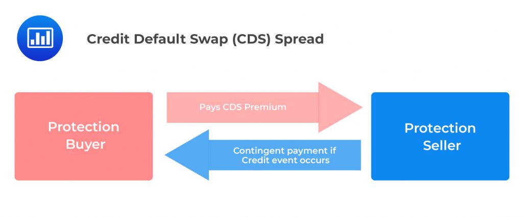
The Credit Default Swap (CDS) basis is a critical financial metric used to calculate payouts following a credit event, such as a default. It provides precise payout calculations without leaving residual interest rate risk, making it essential for traders and investors in managing credit risks. Conversely, the Option-Adjusted Spread (OAS) extends the Z-spread by including options pricing to reflect potential changes due to interest rate volatility, such as the likelihood of a bond being called. This makes the OAS a crucial measure for adjusting a bond’s yield spread over the zero curve to equate its market price, and is particularly valuable for comparing bonds with or without embedded options in an active management setting.
OAS calculations rely on advanced models that incorporate the current term structure of interest rates, volatility, and specific options-related features of bonds. While highly effective, OAS is sensitive to the assumptions made within these models, which can affect its accuracy in predicting returns on complex securities. Despite these theoretical limitations and potential inaccuracies, such as those arising from using constant versus actual prepayment speeds, OAS remains the preferred method for evaluating credit spread risks across various bonds in a portfolio, providing a standardized measure for bonds with embedded options.
FRNs are a unique type of bond that pays a periodic interest coupon, which is a combination of a variable Market Reference Rate (MRR) and a usually constant yield spread. This is in contrast to fixed-rate bonds, which have a fixed yield to maturity (YTM). The interest rate risk differs between these two types of bonds, hence the need to focus on FRN credit spread measures.
Valuing a floating-rate bond is a critical skill for investors. The valuation of a floating-rate bond on a payment date can be represented by the following equation:
$$ \begin{align*} PV & = \frac{(MRR + QM) \times FV \times{m}}{\left(1+ \frac{MRR+DM}{m}\right)^1} + \frac{(MRR + QM) \times FV \times m}{\left(1+ \frac{MRR + DM}{m} \right)^2 } \\ & \ldots + \frac{(MRR + QM) \times FV \times m+FV}{\left(1+\frac{MRR+DM}{m}\right)^N} \end{align*} $$
Where:
PV is the present value of the bond.
MRR is the Market Reference Rate.
QM is the Quoted Margin, which is the yield spread over the MRR established upon issuance to compensate investors for assuming the credit risk of the issuer.
FV is the face value (or par value) of the bond.
m is the number of compounding periods per year.
DM is the Discount Margin, which is the yield spread versus the MRR such that the fixed-rate note (FRN) is priced at par on a rate reset date.
N is the number of periods until maturity.
The Quoted Margin (QM) and the Discount Margin (DM) are two key concepts in understanding FRNs. The QM is a yield spread over the MRR that compensates investors for assuming the credit risk of the issuer. It is usually fixed through maturity and does not reflect credit risk changes over time. The DM, on the other hand, is the yield spread versus the MRR that prices the FRN at par on a rate reset date. If the issuer’s credit risk remains unchanged, the DM equals the QM.
When it comes to bond pricing between coupon dates, the flat price of a bond can either be at a premium or discount to its par value. This depends on whether the Market Required Rate (MRR) falls or rises. For instance, if the MRR falls to 125 basis points due to an issuer upgrade on a reset date, the Floating Rate Note (FRN) will be priced at a premium above par value. This premium is essentially the present value of the premium future cash flows. The annuity difference of 25 basis points per period is calculated for the remaining life of the bond.
The Zero-Discount Margin (Z-DM) is a concept that incorporates forward MRR into the yield spread calculation for FRNs. Similar to the zero-volatility spread for fixed-rate bonds, the Z-DM is a fixed periodic adjustment applied to the FRN pricing model to solve for the observed market price. This calculation incorporates the respective benchmark spot rates derived from the swap or government yield curve for the Z-spread into the FRN pricing model.
$$ \begin{align*} PV & = \frac{(MRR + QM) \times FV}{m \left(1 + \frac{MRR + Z \cdot DM}{m}\right)} + \frac{(\text{z}_2 + QM) \times FV}{m \left(1 + \frac{\text{z}_2 + Z \cdot DM}{m}\right)^2} + \ldots \\ & + \frac{(\text{z}_N + QM) \times FV}{m \left(1 + \frac{\text{z}_N + Z \cdot DM}{m}\right)^N} + FV \end{align*} $$
Where:
\(MRR\) is the Market Reference Rate.
\(QM\) is the Quoted Margin, the yield spread over the MRR established upon issuance to compensate investors for assuming the credit risk of the issuer.
\(FV\) is the face value (or par value) of the bond.
\(m\) is the number of compounding periods per year.
\(Z \cdot DM\) is the product of the zero-discount margin and Discount Margin, affecting the rate adjustment over the period.
\(\text{z}_2, \ldots, \text{z}_N\) represent different period-specific rates that could be seen as phase-adjusted rates or specific benchmarks for those periods.
\(N\) is the number of periods until maturity.
The primary focus is on roll-down return and E (Δ Price due to investor’s view of yield spreads). These variables are crucial for active managers who strive to outperform a benchmark portfolio using credit strategies.
Roll-down return is a concept that encapsulates the accumulation of coupon income and additional return from fixed-rate bond price appreciation over an investment horizon, assuming positive benchmark rates and an upward sloping yield curve. For instance, consider a corporate bond priced at a spread over a government bond. The return from coupon income would be higher by the bond’s original credit spread. The roll-down return due to price appreciation will also be higher because the higher-yielding instrument will generate greater carry over time. However, it’s crucial to understand that this higher return is accompanied by greater risk and assumes all promised payments are made, and the bond remains outstanding—meaning, no default or prepayment occurs, and the bond is not called.
Active credit managers often isolate the E (\(\Delta\) Price due to investor’s view of yield spreads) term in Equation 1 as they manage benchmark rate risks separately from credit.
$$ \begin{align*} \% \Delta PV_{\text{Spread}} & \approx -(\text{EffSpreadDur} \times \Delta \text{Spread}) \\ & + \left(\frac{1}{2} \times \text{EffSpreadCon} \times (\Delta \text{Spread})^2\right) \end{align*} $$
where \(\text{EffSpreadDur}\) is the effective spread duration, EffSpreadCon is the effective spread convexity, and \(\Delta \text{Spread}\) is typically defined as the change in OAS.
$$\text{EffSpreadDur} = \frac{(PV) – (PV_+)}{2 \times (\Delta \text{Spread}) \times (PV_0)}$$
$$\text{EffSpreadCon} = \frac{(PV) + (PV_+) – 2 \times (PV_0)}{(\Delta \text{Spread})^2 \times (PV_0)}$$
Active bond portfolio managers often estimate the changes in bond portfolio value due to spread changes. This is done by substituting market value-weighted averages for duration and convexity measures. It’s crucial to understand that spread changes for lower-rated bonds are usually consistent on a proportional percentage rather than an absolute basis. This necessitates the adjustment of spread duration to capture the Duration Times Spread (DTS) effect.
The DTS of a portfolio is calculated as the market value-weighted average of the DTS of its individual bonds. Spread changes of a portfolio are measured on a percentage basis rather than in absolute basis point terms. Active credit managers often use spread duration-based statistics to gauge the first-order impact of spread movements when considering the incremental effects of credit-based portfolio decisions.
$$DTS \approx (\text{EffSpreadDur} \times \text{Spread})$$
$$\text{ExcessSpread} \approx \text{Spread}_0 – (\text{EffSpreadDur} \times \Delta \text{Spread})$$
When a bond issuer’s likelihood of default increases, the expected future cash flows from the bond decrease. This leads to the bond’s value nearing the present value of the expected recovery. For instance, if a company’s financial health deteriorates, the risk of default on its bonds increases, reducing the bond’s value.
The annualized expected excess return is a measure of the return on a bond over and above the risk-free rate.
$$ \begin{align*} E [\text{ExcessSpreadReturn}] & \approx \text{Spread}_0 − (\text{EffSpreadDur} \times \Delta \text{Spread}) \\ & − (\text{POD} \times \text{LGD}) \end{align*} $$
Where:
\(\text{E[ExcessSpreadReturn]}\) is the expected excess spread return.
\(\text{Spread}\) is the yield spread over the risk-free rate.
\(\text{EffSpreadDur}\) is the effective spread duration.
\(\Delta \text{Spread}\) is the change in spread.
\(\text{POD}\) is the probability of default.
\(\text{LGD}\) is the loss given default.
Active credit management aims to maximize the expected spread return while minimizing the portfolio credit loss. This is the percentage of the par value lost to defaults over time.
Duration measures the sensitivity of a bond’s price to changes in interest rates. For Floating Rate Notes (FRNs), the duration is near zero when trading at par on a reset date due to the periodic reset of the Marginal Rate of Return (MRR).
For FRNs, changes in spread are the primary driver of price changes. The formulas for the effective rate duration and effective spread duration are as follows:
$$\text{EffRateDur}_{FRN} = \frac{(PV_-) – (PV_+)}{2 \times (\Delta MRR) \times (PV_0)}$$
$$\text{EffSpreadDur}_{FRN} = \frac{(PV_-) – (PV_+)}{2 \times (\Delta DM) \times (PV_0)}$$
Where:
\(\text{EffRateDur}_{\text{FRN}}\) is the effective interest rate duration for floating rate notes.
\(PV\) and \(PV_+\) represent the present values before and after a small change in the rate, respectively.
\(\Delta MRR\) is the change in the market reference rate.
\(PV_0\) is the present value at the baseline time period.
\(\text{EffSpreadDur}_{\text{FRN}}\) is the effective interest spread duration for floating rate notes.
\(\Delta DM\) is the change in discount margin.
Practice Questions
Question 1: Which of the following statements is most accurate about the factors that influence the expected return of a fixed-income security and the risks associated with it?
- The yield spread primarily compensates investors for assuming market and interest rate risks.
- Credit risk for a specific borrower depends solely on the likelihood of default and the loss severity in a default scenario.
- Liquidity risk refers to an investor’s ability to readily buy or sell a specific security and can influence the Yield to Maturity difference between the purchase and sale price of a bond.
Answer: Choice C is correct.
Liquidity risk refers to an investor’s ability to readily buy or sell a specific security without causing a significant change in its price and can influence the Yield to Maturity difference between the purchase and sale price of a bond. Liquidity risk is a significant factor that influences the expected return of a fixed-income security. It is the risk that an investor might not be able to buy or sell a bond quickly enough when they want to, without significantly affecting the bond’s price. This risk can affect the yield to maturity (YTM) difference between the purchase and sale price of a bond. If a bond is illiquid, the investor might have to sell it at a discount (lower price), which increases the YTM. Conversely, if a bond is highly liquid, the investor might be able to sell it at a premium (higher price), which decreases the YTM. Therefore, liquidity risk can influence the expected return of a fixed-income security.
Choice A is incorrect. The yield spread primarily compensates investors for assuming credit risk, not market and interest rate risks. The yield spread is the difference in yield between a risk-free government bond and a riskier bond, such as a corporate bond. This spread compensates investors for the additional risk they take on when they invest in the riskier bond. While market and interest rate risks can influence the yield spread, they are not the primary factors that the spread compensates for.
Choice B is incorrect. Credit risk for a specific borrower does not depend solely on the likelihood of default and the loss severity in a default scenario. While these are important factors, credit risk also depends on other factors such as the borrower’s creditworthiness, the terms of the bond, and the overall economic environment. Therefore, this statement is not the most accurate description of the factors that influence the expected return of a fixed-income security and the risks associated with it.
Question 2: Which of the following statements is correct regarding the yield spreads as a percentage of total YTM for different rated issuers over the period from mid-2009 to mid-2020?
- The yield spread as a percentage of total YTM was highest for A rated issuers.
- On average, 60% of total YTM was attributable to yield spread for BB rated issuers as compared to 33% for A rated issuers.
- The yield spread as a percentage of total YTM was lowest for BB rated issuers.
Answer: Choice B is correct.
On average, 60% of total Yield to Maturity (YTM) was attributable to yield spread for BB rated issuers as compared to 33% for A rated issuers. This statement is correct because yield spreads over default risk-free government bonds are a significant factor in credit risk considerations. They serve as a compensation for investors against the potential risk of not receiving the promised cash flows due to issuer default and the severity of loss if such a default occurs. These spreads can vary significantly across different ratings categories and time periods. For instance, the yield spreads as a percentage of total Yield to Maturity (YTM) for A-, BBB-, and BB rated US corporate issuers from mid-2009 to mid-2020 were considered. In this context, the yield spread as a percentage of total YTM was highest for BB rated issuers, not A rated issuers. This is because BB rated issuers have a higher credit risk compared to A rated issuers, and therefore, investors require a higher yield spread to compensate for this increased risk.
Choice A is incorrect. The yield spread as a percentage of total YTM was not highest for A rated issuers. A rated issuers have a lower credit risk compared to BB rated issuers, and therefore, the yield spread as a percentage of total YTM would be lower for A rated issuers.
Choice C is incorrect. The yield spread as a percentage of total YTM was not lowest for BB rated issuers. BB rated issuers have a higher credit risk compared to A rated issuers, and therefore, the yield spread as a percentage of total YTM would be higher for BB rated issuers.
Portfolio Management Pathway Volume 2: Learning Module 6: Fixed-Income Active Management: Credit Strategies.
LOS 6(a): Discuss bottom-up approaches to credit strategies.
LOS 6(b): Discuss the advantages and disadvantages of credit spread measures for spread-based fixed-income portfolios, and explain why option-adjusted spread is considered the most appropriate measure
Offered by AnalystPrep


Get Ahead on Your Study Prep This Cyber Monday! Save 35% on all CFA® and FRM® Unlimited Packages. Use code CYBERMONDAY at checkout. Offer ends Dec 1st.